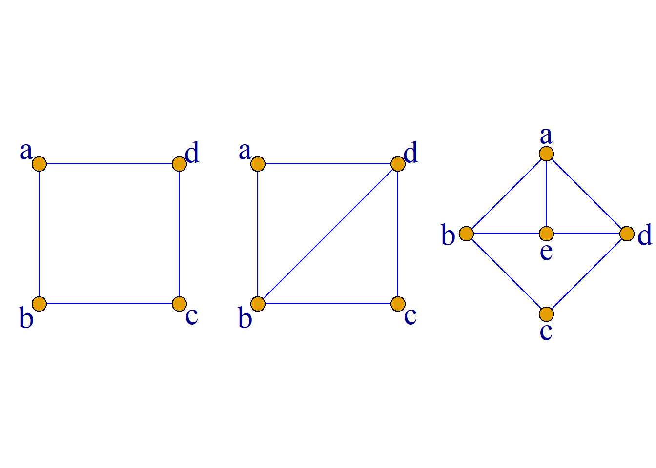
Other Graphs
Eulerian Graphs
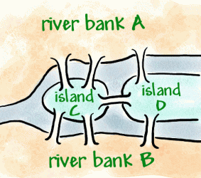
Graph theory originated in the 18th century. In 1736, the Swiss mathematician Euler published the first paper on graph theory, “The Seven Bridges of Königsberg Problem”.
Eulerian traversal: a closed walk that traverses every edge of the graph at least once.
Eulerian circuit: a closed walk that traverses each edge exactly once. A graph containing an Eulerian circuit is called an Eulerian graph.
Similarly, a trail that traverses each edge of the graph is called an Eulerian trail.
These terms are named after Euler because in 1736 Euler solved the famous Seven Bridges of Königsberg problem.
Definition: For a graph \(G\), a walk that traverses each edge exactly once is called an Eulerian trail (or Euler path). A graph that has an Eulerian trail is called a semi-Eulerian graph.
A circuit that traverses each edge in the graph exactly once is called an Eulerian circuit of the graph, and a graph with an Eulerian circuit is called an Eulerian graph.
Obviously, the Euler path is a simple path that passes through all the edges in the graph, and the Euler circuit is a simple cycle that passes through all the edges in the graph.
Semi-Eulerian graph vs. Eulerian graph: one has an Eulerian trail, while the other has an Eulerian circuit.
Whether a graph has an Eulerian trail (or Eulerian circuit) is equivalent to whether it can be drawn in one stroke.
If the pen does not leave the paper and each edge is drawn exactly once, then returning to the starting point means the graph is Eulerian; otherwise it is semi-Eulerian.
- You can draw in one stroke and then return to the starting point; (b) You can draw in one stroke, but the pen cannot return to the starting point; (c) You cannot draw all the edges in one stroke at all.
There is a simple method to determine whether there is an Euler path or an Euler circuit in a graph. Euler discovered this method and proved it while solving the Seven Bridges of Königsberg problem.
Theorem: Suppose the undirected graph \(G={\langle}V, E{\rangle}\) is connected, then
There is an Eulerian circuit in \(G\) if and only if the degrees of all vertices in \(G\) are even.
There is an Euler path but no Euler circuit in \(G\), if and only if the degree of exactly two nodes in \(G\) is odd.
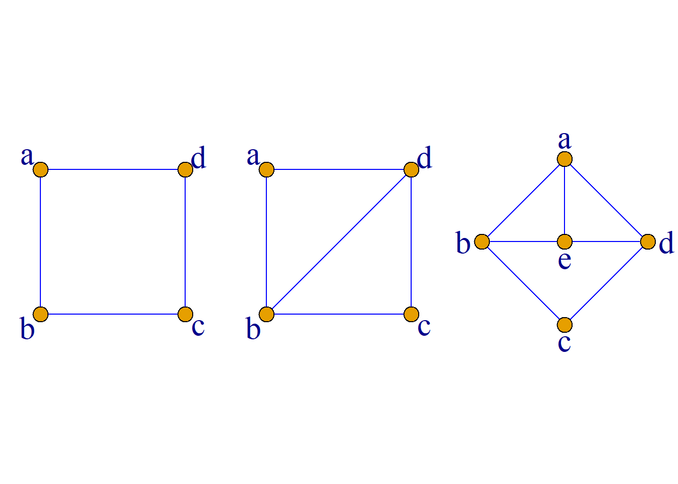
Example: Determine whether there are Euler paths and Euler circuits in figures (a), (b), and (c).
Solution: Figure (a), \(d(a)=d(b)=d(c)=d(d)=2\), the degrees of all vertices are even, so there is an Euler circuit;
Figure (b), \(d(a)=d(c)=2, d(b)=d(d)=3\), there are two vertices with odd degrees, so there is an Euler path;
Figure (c), \(d(a)=d(b)=d(d)=d(e)=3, d(c)=2\), there are 4 vertices with odd degrees, so there is neither an Euler path nor an Euler circuit.
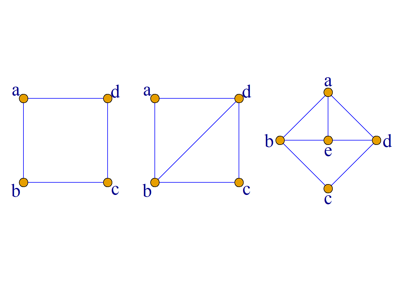
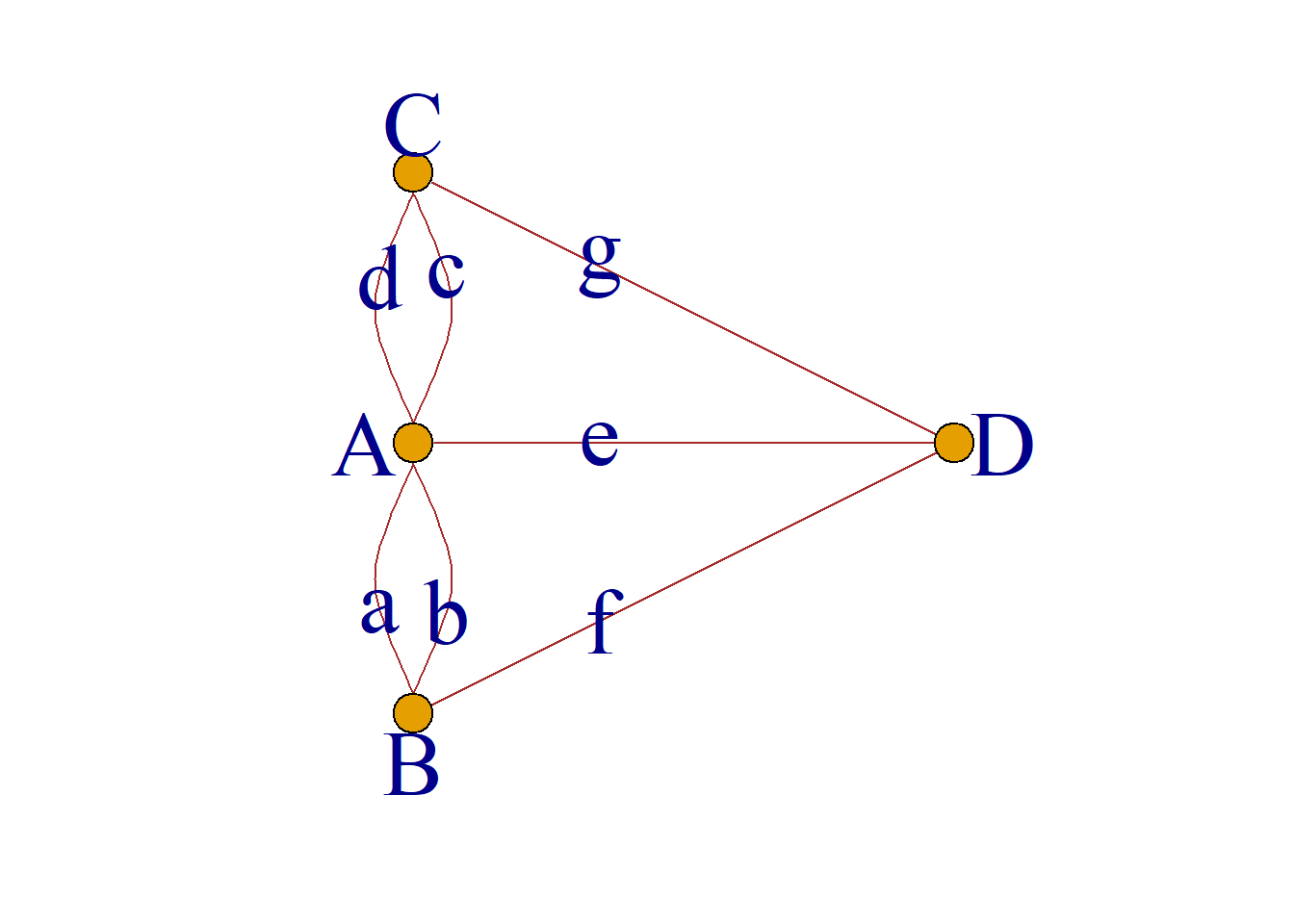
Seven Bridges Problem:
\(d(A)=5\)
\(d(B)=3\)
\(d(C)=3\)
\(d(D)=3\)
The degrees of the four nodes are all odd, so there is no Eulerian circuit, and the seven-bridge problem has no solution.
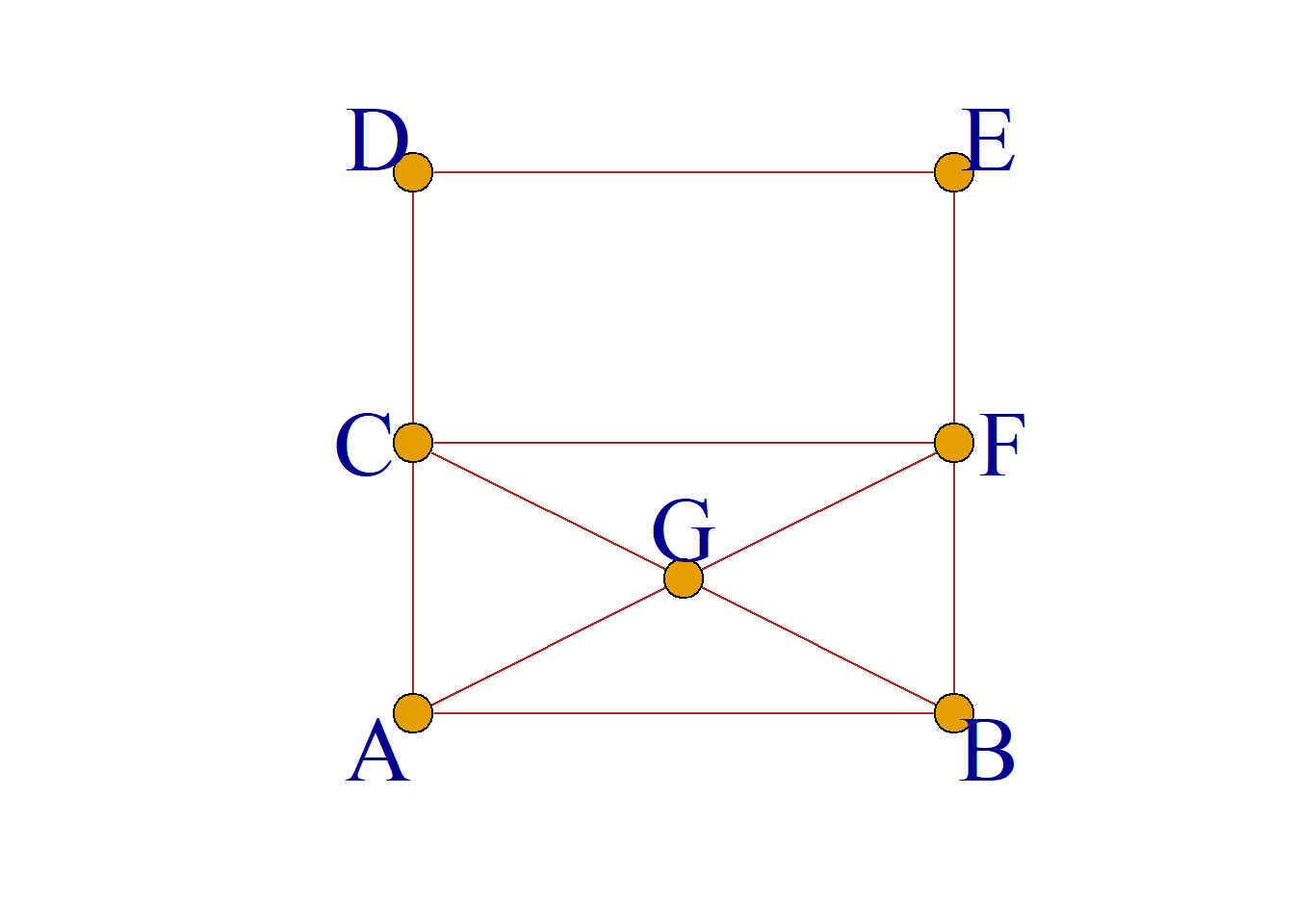
Example: The picture shows a street graph. The sprinkler truck starts from point \(A\) to perform the watering task. Let’s ask if there is a sprinkler line that allows the sprinkler truck to pass through all streets without repeating and finally return to garage \(B\).
Solution: This question is to find out whether there is an Euler path from \(A\) to \(B\) in the graph. Since only \(A\) and \(B\) are odd-degree nodes, such a sprinkler route exists, such as:
\(ACDEFBGCFGAB\)
or
\(AGFEDCFBGCAB.\)
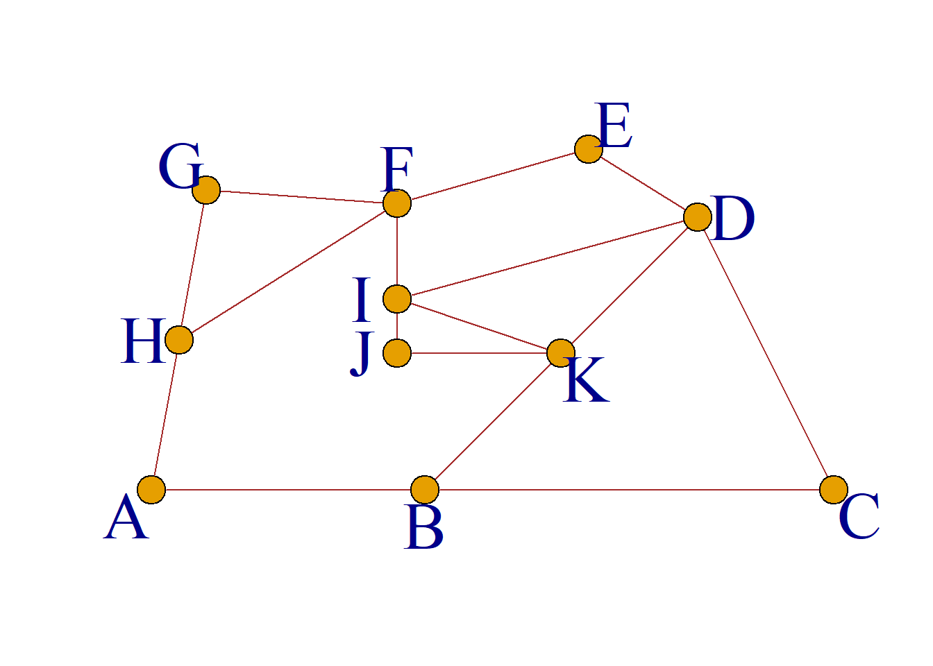
Example: “Two ants race problem”. Two ants A and B are located at nodes \(A\) and \(B\) of graph \(G\) respectively, and assume that the lengths of all sides in the graph are equal. A proposes a competition with B: starting from the node where they are located, walking through all the edges in the graph and finally returning to node \(C\). If they have the same speed, who reaches the destination first?
Solution: In the graph \(G\), there are only two odd-degree nodes \(B\) and \(C\), so there is an Euler path whose starting point and end point are \(B\) and \(C\). Ant B can take an Euler path from \(B\) to \(C\), with the number of edges being 9. If Ant A wants to go through all the edges in the graph to reach \(C\), it must first take at least one edge to reach \(B\), and then take an Euler path. It must take at least 10 edges to reach \(C\), so Ant B must win.
Example: The floor plan of a park is as shown in the figure. Can visitors travel through every road without repeating it? Where should entrances and exits be located?
Solution: Points \(H\) and \(B\) are nodes with odd degrees, and the degrees of the other nodes are all even. Therefore, the entrance and exit are set at \(H\) and \(B\), and tourists can walk every road without duplication.
In fact, the Euler path is the shortest path that passes through all the edges in the graph; the Euler circuit is the shortest path that passes through all the edges in the graph.
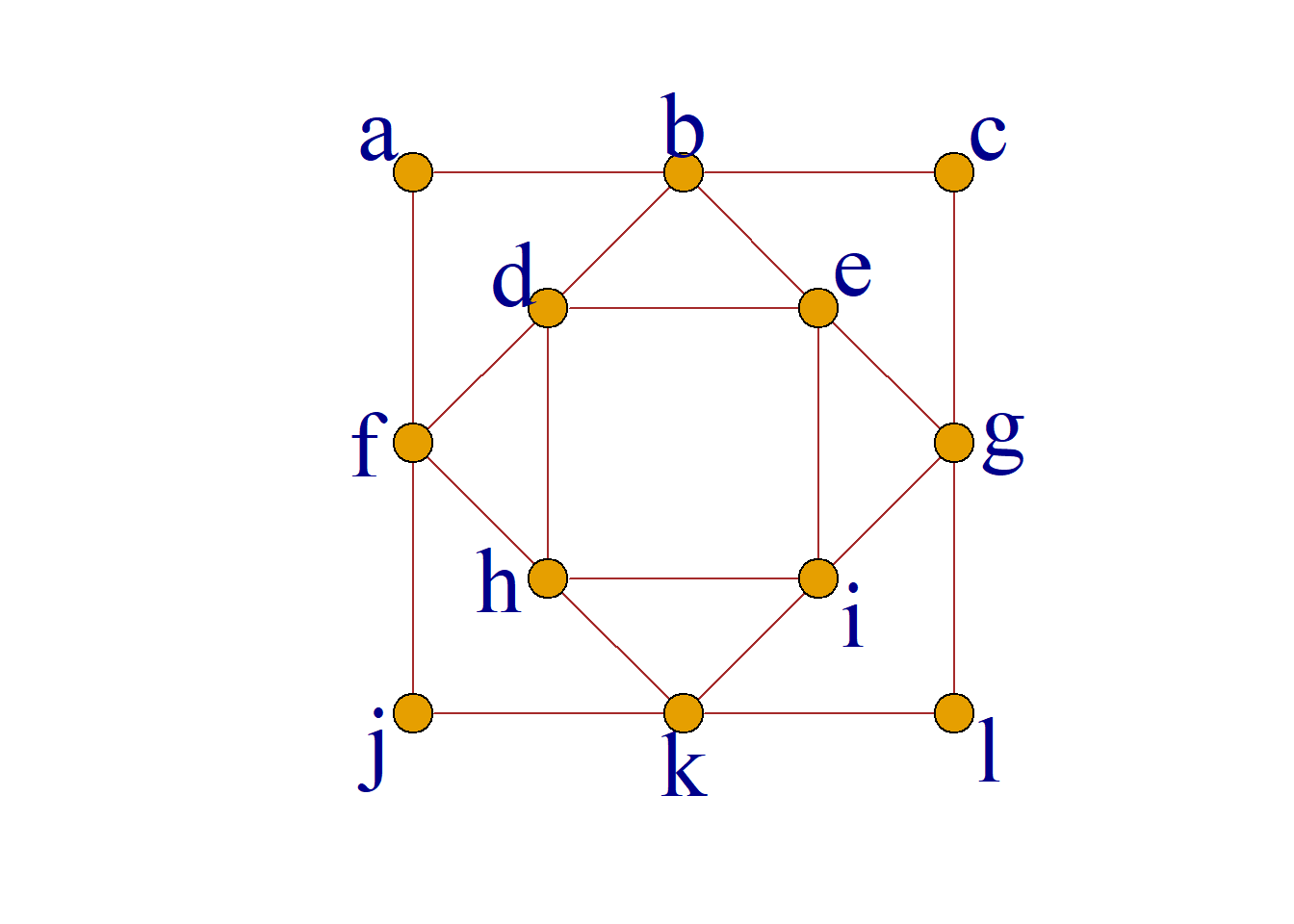
Example: For the street shown in the picture, is there a delivery route that allows the postman to start from \(a\) and pass through all the streets once before returning to the post office \(a\)?
The degrees of all vertices are even, so there is an Eulerian circuit, which is the required delivery route. For example: afjklgcbdfhkigedhieba.
Fleury algorithm to find Euler circuit
Theorem: Let Fleury’s algorithm: Let Eulerian graph \[G={\langle}V, E{\rangle}\]
1 Take \(v_0{\in}V\) arbitrarily, let \(P_0=v_0\);
2 Assume that the path \(p_i = v_0e_1v_1e_2{\cdots}e_iv_i\) has been traveled, and select \(e_{i+1}\) from \(E\)-\(\{e_1, e_2, e_3, {\cdots}, e_i\}\) as follows:
\(e_{i+1}\) is associated with \(v_i\);
Unless there is no other edge to go, \(e_{i+1}\) should not be \(G_i = bridge in G-\{e_1, e_2, e_3, {\cdots}, e_i\}\).
3 When 2 can no longer be performed, the algorithm stops.
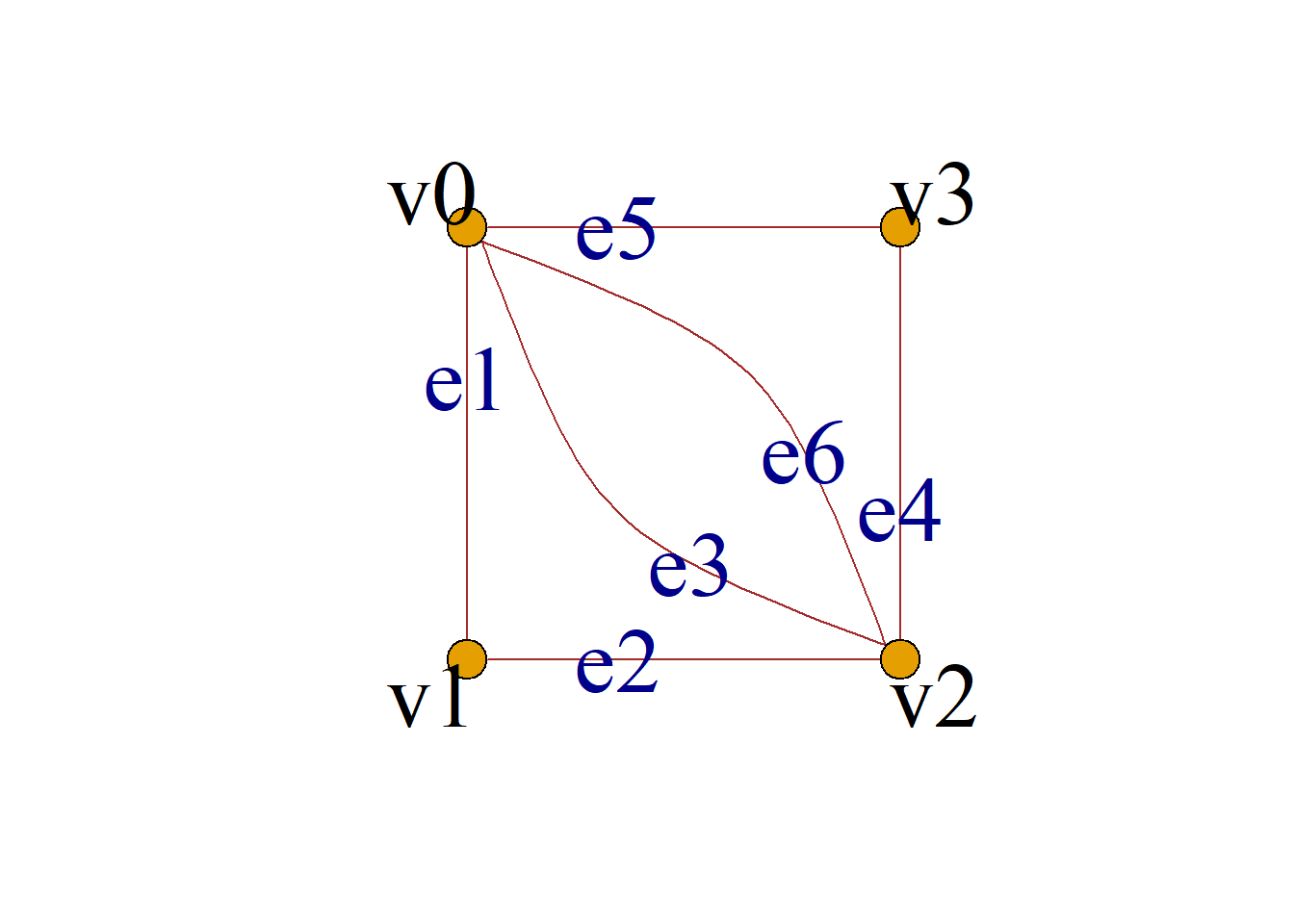
Example: Use Fleury’s algorithm to find an Euler circuit such as \(G={\langle}V, E{\rangle}\).
Solution: Take any \(v_0{\in}V\).
Choose \(e_1\), get \(v_0e_1v_1\)
Choose \(e_2\), get \(v_0e_1v_1 e_2v_2\)
Choose \(e_6\), get \(v_0e_1v_1 e_2v_2 e_6v_0\)
Choose \(e_3\), get \(v_0e_1v_1 e_2v_2 e_5v_0 e_3v_2\)
Choose \(e_4\), get \(v_0e_1v_1 e_2v_2 e_5v_0 e_3v_2 e_4v_3\)
Choose \(e_5\), get \(v_0e_1v_1 e_2v_2 e_5v_0 e_3v_2 e_4v_3 e_5v_0\)
Theorem: Let \(G\) be a non-trivial Eulerian graph if and only if \(G\) is connected and is the union of several simple cycles with non-repeating edges.
Theorem: Suppose the directed graph \(G={\langle}V, E{\rangle}\) is weakly connected, then:
There is an Eulerian circuit in \(G\) if and only if the in-degree of each vertex in \(G\) is equal to its out-degree.
There is an Euler path but no Euler circuit in \(G\), if and only if, except for two nodes in \(G\), the in-degree of the remaining nodes is equal to the out-degree, and among the two excepted nodes, the in-degree of one node is 1 greater than the out-degree, and the in-degree of the other node is 1 smaller than the out-degree.
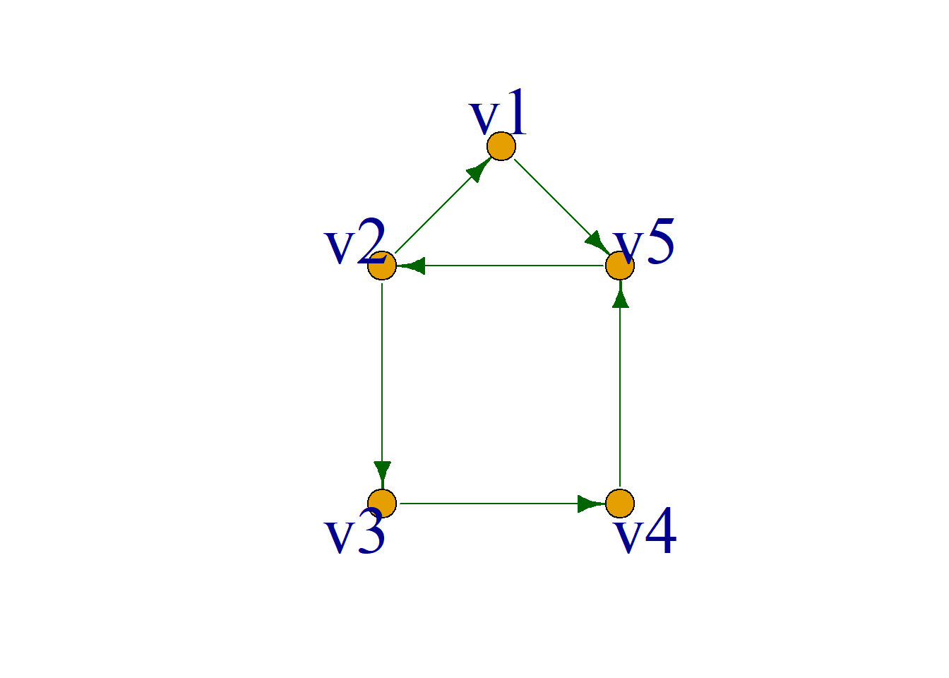
Example: Determine whether the graph contains Euler paths and Euler circuits.
Solution: For \(G\), \[d^+(v_1)=1, d^-(v_1)=1\] \[d^+(v_2)=2, d^-(v_2)=1\] \[d^+(v_3)=1, d^-(v_3)=1\] \[d^+(v_4)=1, d^-(v_4)=1\] \[d^+(v_5)=1, d^-(v_2)=2\] Therefore, there is an Euler path, such as \(v_2v_3v_4v_5v_2v_1v_5\).
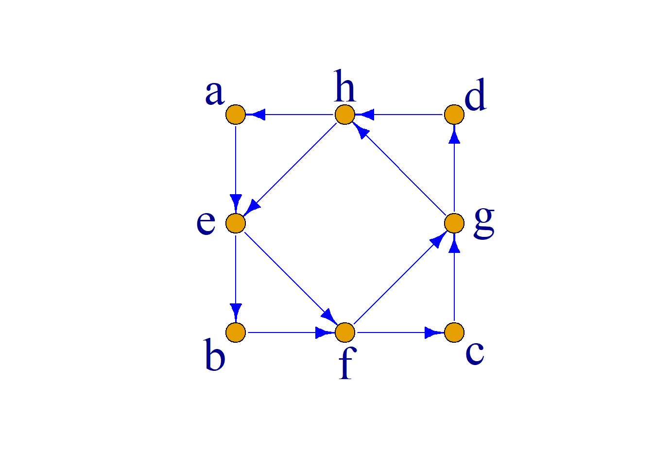
Example: Determine whether there is an Euler path or an Euler circuit in the figure below.
Solution: For \(G\), \[d^+(a)=d^-(a)=1 , d^+(b)=d^-(b)=1\] \[d^+(c)=d^-(c)=1, d^+(d)=d^-(d)=1\] \[d^+(e)=d^-(e)=2, d^+(f)=d^-(f)=2\] \[d^+(g)=d^-(g)=2, d^+(h)=d^-(h)=2\]
Therefore, there is an Euler circuit.
Hamiltonian Graphs
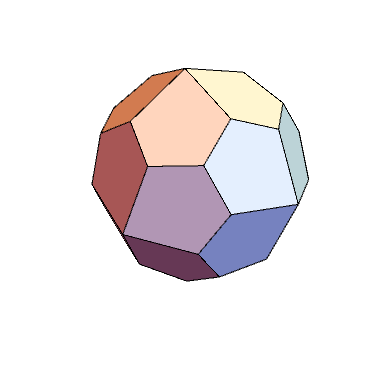
The Hamiltonian graph originated from a mathematical game, which was the “Around the World Problem” proposed by the Irish mathematician Hamilton in 1859:
Use the 20 vertices of a regular dodecahedron to represent 20 famous cities in the world. It is required to start from a city along the edges of the regular dodecahedron, pass through each city exactly once, and then return to the starting point.
Unlike the Seven Bridges of Königsberg problem, Mr. Hamilton soon received answers from all over the world to solve the problem of traveling around the world.
Definition: For graph \(G\), a path that passes through each node in the graph once and only once is called a Hamiltonian path of the graph. A cycle that passes through each node in the graph once and only once is called a Hamiltonian cycle of the graph, and a graph with a Hamiltonian cycle is called a Hamiltonian graph.
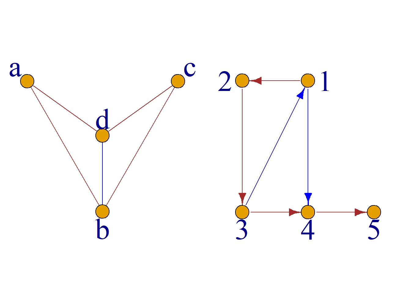
As shown in the picture:
There are Hamiltonian paths and Hamiltonian circuits in (a). A Hamiltonian path is \((a, b, c, d)\), and a Hamiltonian circuit is \((a, b, c, d, a)\).
There is also a Hamiltonian path in (b). A Hamiltonian path is \((1, 2, 3, 4, 5)\), and there is no Hamiltonian cycle.
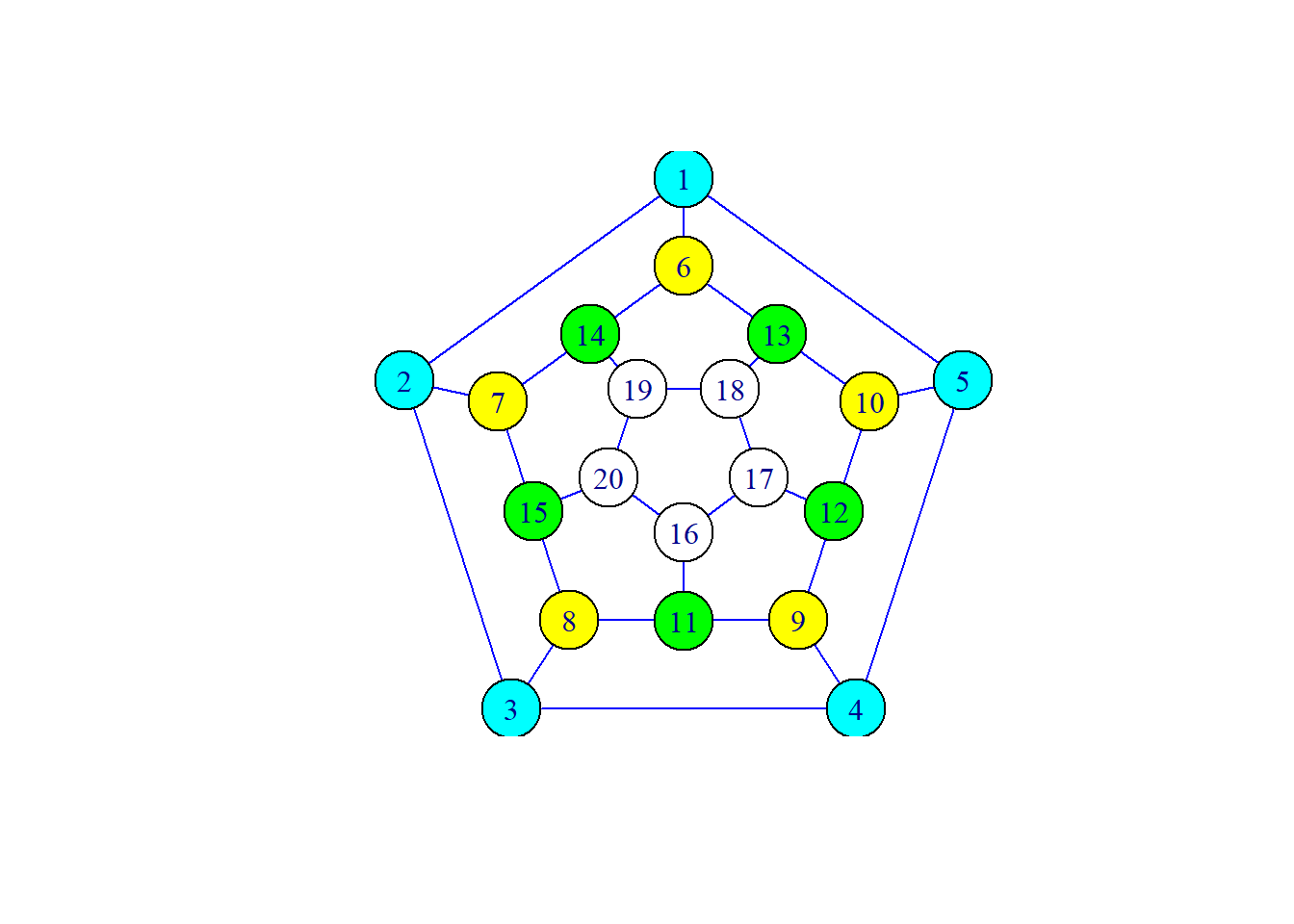
There is a Hamiltonian cycle in the regular dodecahedron, which can travel around, for example: \(1\, 2\, 3\, 10\, 12\, 9\, 4\, 3\, 8\, 11\, {\cdots}20\, 6\).
Unlike the case of the Eulerian graph, so far, the necessary and sufficient conditions to judge that the Hamiltonian cycle is non-trivial are not clear yet.
In fact, this is one of the major unsolved problems in graph theory.
But there are some sufficient or necessary conditions for Hamiltonian graphs.
Theorem: Suppose the undirected graph \(G={\langle}V, E{\rangle}\) is a Hamiltonian graph, then for every non-empty proper subset \(S\) of the node set \(V\): \[p(G-S){\leq}|S|\] Where \(p(G-S)\) is the number of connected branches of \(G-S\).
Proof: Because \(G\) is a Hamiltonian graph, there is a Hamiltonian cycle in \(G\).
Suppose \(C\) is such a Hamiltonian cycle, obviously there is \(p(C-S){\leq}|S|\).
And \(C-S\) is the generated subgraph of \(G-S\), so \(p(G-S){\leq}p(C-S)\), so there is \(p(G-S){\leq}|S|\).
This theorem gives a necessary condition for an undirected graph to be a Hamiltonian graph, but it is not a sufficient condition.
Corollary: Assume that the undirected graph \(G={\langle}V, E{\rangle}\) has a Hamiltonian path, then for every non-empty proper subset \(S\) of the node set \(V\): \[p(G-S){\leq}|S|+1\] Where \(p(G-S)\) is the number of connected branches of \(G-S\).
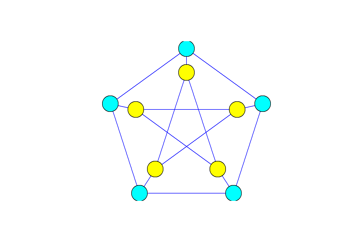
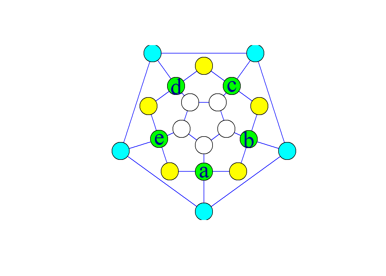
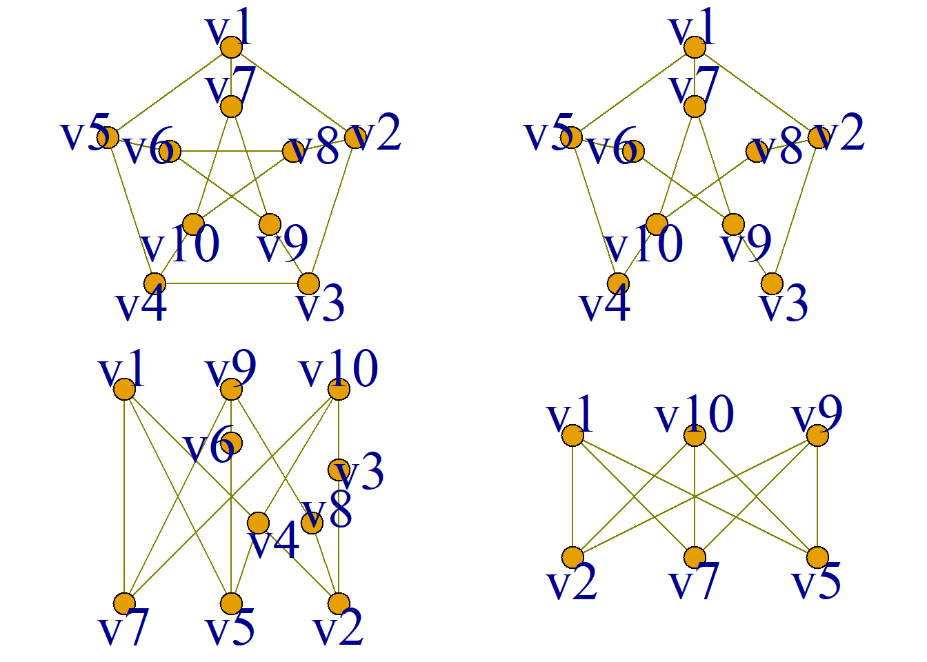
The Petersen diagram in the figure satisfies \[p(G-S){\leq}|S|,\] However, this graph is not a Hamiltonian graph.
However, a graph that does not satisfy this condition must not be a Hamiltonian graph, so it can be used to prove that some graphs are not Hamiltonian graphs.
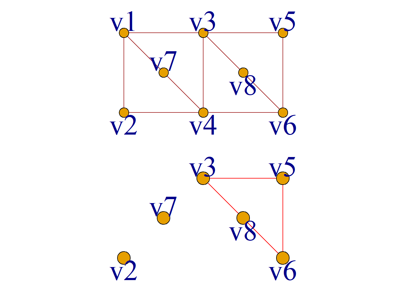
Example: An undirected graph as shown in Figure \(G\):
Take \(S=\{v_1, v_4\}\), then:
\(p(G-S)=3>|S|=2.\)
Therefore this undirected graph is not a Hamiltonian graph.
It exists a Hamiltonian path, for example: \(v_2v_4v_7v_1v_3v_8v_6v_5\).
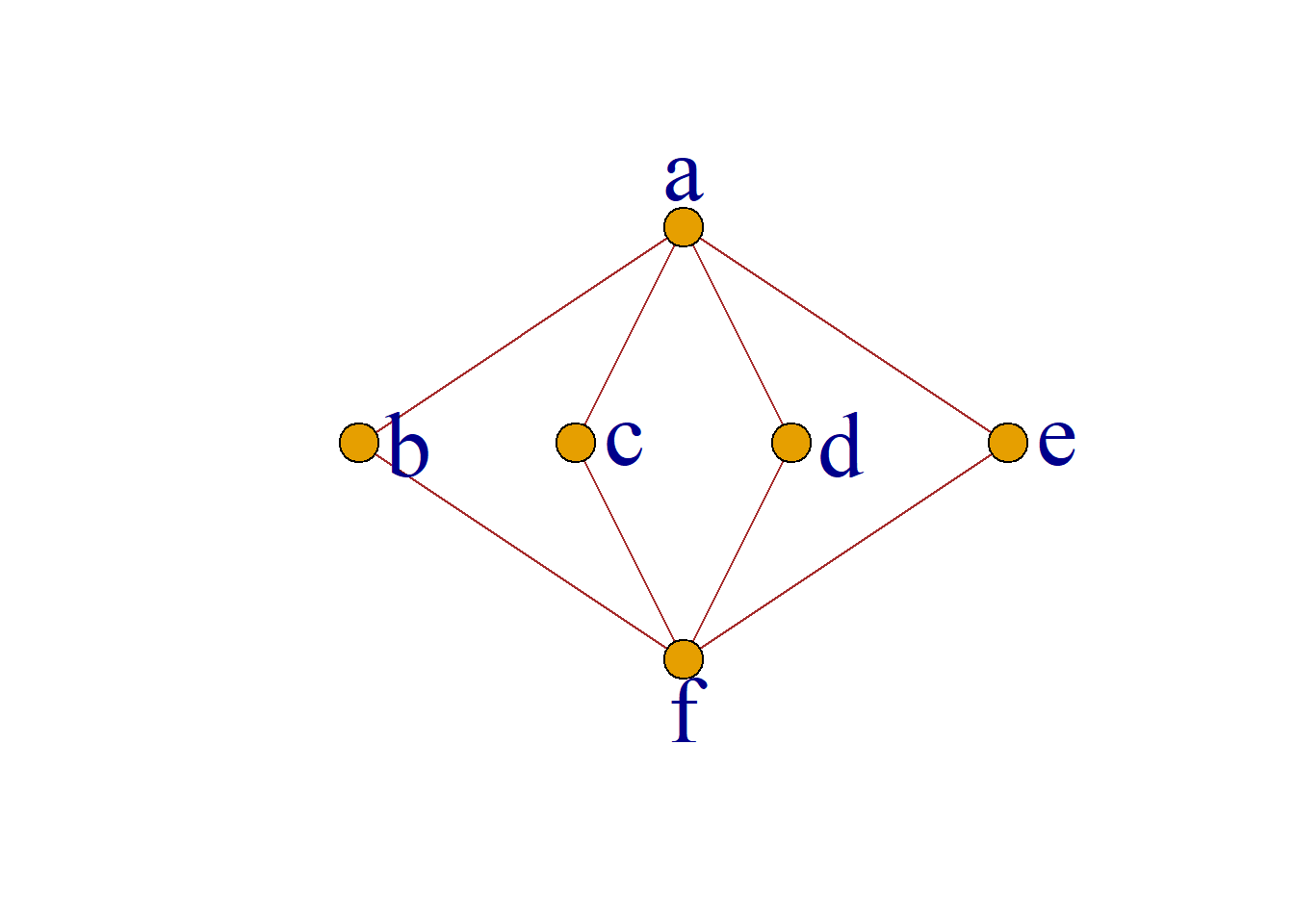
Example: Is the undirected graph shown in Figure \(G\) a Hamiltonian graph or does a Hamiltonian path exist?
Solution: Take \(S=\{a, f\}\), then: \[p(G-S)=4>|S|=2\] dissatisfied
\(p(G-S){\leq}|S|\)
or
\(p(G-S){\leq}|S|+1.\)
Therefore, this undirected graph is not a Hamiltonian graph, and there is no Hamiltonian path.
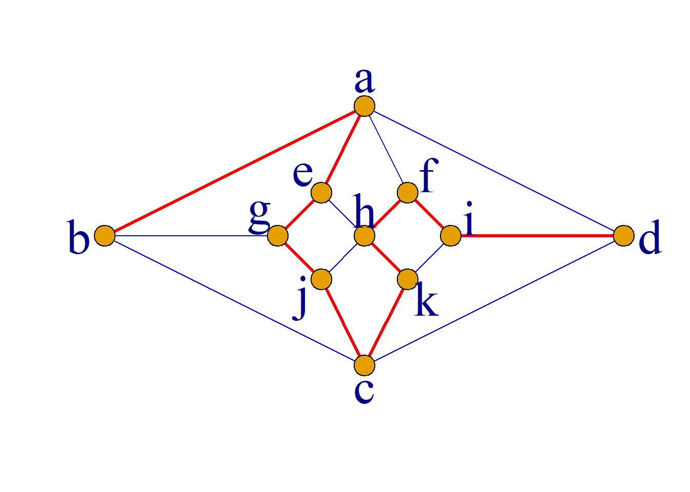
Example: Graph \(G\) is as shown in the figure, determine whether it is a Hamiltonian graph or whether there is a Hamiltonian path?
Solution: Suppose \(V_1=\{a, g, h, i, c\}\), \(V_2=\{b, e, f, j, k, d\}\), then \(p(G-V_1)=|V_2|=6>|V_1|=5\), it can be seen that \(G\) is not a Hamiltonian graph.
But there is a Hamiltonian path.
\(baegjckhfid\) is a Hamiltonian path.
Example: Among the following figures, which ones are Hamiltonian graphs, and which ones have Hamiltonian paths?
Solution:
- For \(G_1\), assume \(V_1=\{a, b, c, d, e\}\), then: \(p(G_1-V_1)=7>|V_1|=5\).
It can be seen that \(G_1\) is not a Hamiltonian graph, and there is no Hamiltonian path.
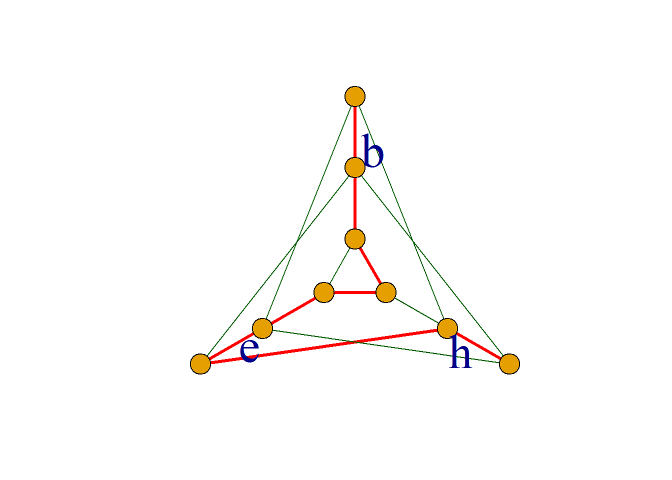
- For \(G_2\), assume \(V_1=\{b, e, h\}\), delete \(V_1\) from the graph to get 4 connected branches, then \(p(G_2-V_1)=4>|V_1|=3\).
It can be seen that \(G_2\) is not a Hamiltonian graph.
But there is a Hamiltonian path.
Theorem: Assume that graph \(G\) is a simple undirected graph with \(n\) nodes. If the sum of the degrees of each pair of nodes in \(G\) is greater than or equal to \(n-1\), then there is a Hamiltonian path (path) in \(G\).
The theorem gives only sufficient conditions, not necessary conditions.
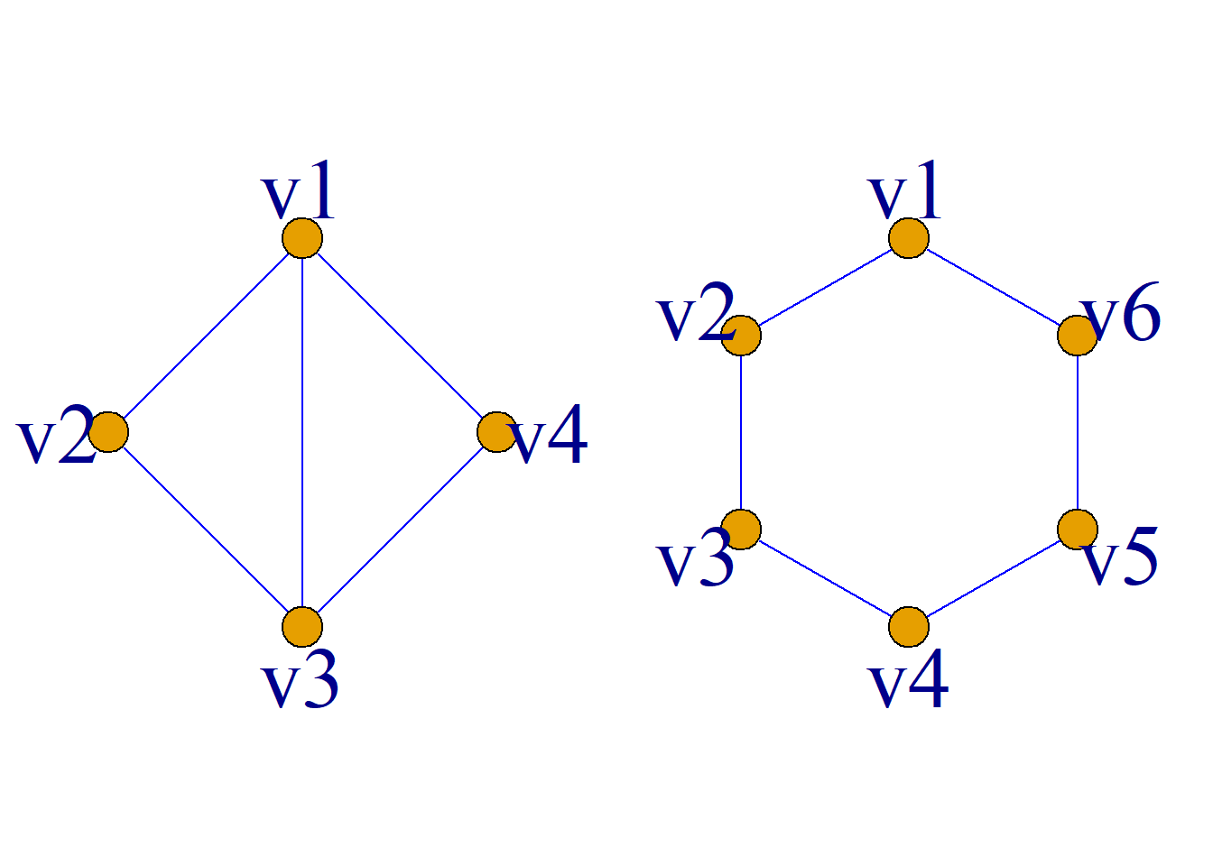
For example, in graph \(G_1\), the sum of the degrees of any two nodes is \({\geq}n-1=3\), so there is a Hamiltonian path; in graph \(G_2\), although the sum of the degrees of any two nodes is \(4<n-1=5\), there is still a Hamiltonian path in the graph.
Theorem: Suppose the graph \(G\) is a simple undirected graph with \(n(n{\geq}3)\) nodes. If the sum of the degrees of each pair of nodes in \(G\) is greater than or equal to \(n\), then \(G\) is a Hamiltonian graph.
The theorem gives only sufficient conditions, not necessary conditions.
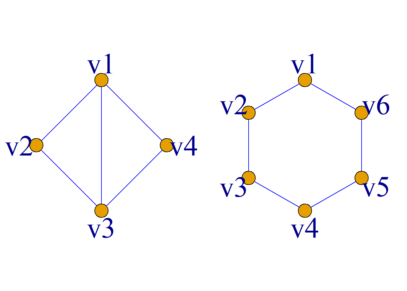
For example, in the graph \(G_1\), the sum of the degrees of any two nodes is \({\geq}n=4\), so there is a Hamiltonian cycle; in the graph \(G_2\), although the sum of the degrees of any two nodes is \(4<n=6\), there is still a Hamiltonian cycle in the graph.
Corollary: Suppose the graph \(G\) is a simple undirected graph with \(n(n{\geq}3)\) nodes. If the degree of each node in \(G\) is greater than or equal to \(n/2\), then \(G\) is a Hamiltonian graph.
Proof: Because the degree of each node in \(G\) is greater than or equal to \(n/2\), the sum of the degrees of any two nodes is greater than or equal to \(n\). According to the previous theorem, \(G\) is a Hamiltonian graph.
Theorem: An undirected complete graph with \(n(n{\geq}3)\) nodes is a Hamiltonian graph.
Theorem: Suppose the graph \(G\) is a directed graph with \(n(n{\geq}2)\) nodes. If all directed edges are replaced by undirected edges, and the resulting undirected graph contains a generated subgraph \(K_n\), then the directed graph \(G\) has a Hamiltonian path.
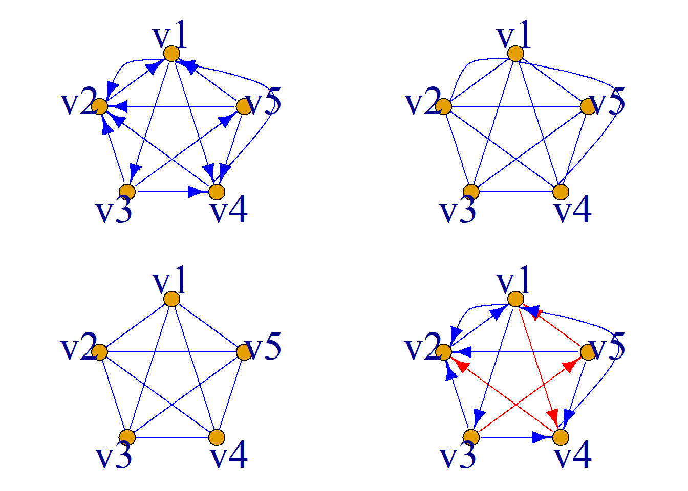
Chinese Postman Problem (CPP)
The postman starts from the post office with the mail to be distributed, passes through each street to be distributed, and returns to the post office after delivering the mail. If he must walk through every street in his jurisdiction at least once, how to choose the delivery route so that the postman walks as little distance as possible.
This problem was first raised by Chinese mathematician Mr. Guan Meigu (Professor of the Department of Mathematics at Shandong Normal University) in 1962, so it is known internationally as the Chinese Postman Problem.
In social activities, we often encounter such problems, such as: Every day, water trucks in the streets and all kinds of express delivery for online shopping need to solve the problem of the shortest distance to walk.
Definition: Suppose \(G={\langle}V, E{\rangle}\) is an undirected graph. If each edge \(e\) of \(G\) is assigned a positive real number \(W(e)\), then \(G\) is called an undirected weighted graph (or simply a weighted graph), and \(W(e)\) is called the weight of edge \(e\).
Regulation: For \(v_i{\in}V\), then \(W(v_i, v_i)=0\); For \(v_i, v_j{\in}V\), if \((v_i, v_j){\notin}E\), then \(W(v_i, v_j)=\infty\).
The weighted graph is recorded as \(G={\langle}V, E, W{\rangle}\). In the weighted graph, the weight of the edge is also called the length of the edge. At this time, the length of a path refers to the sum of the lengths of each edge in the path.
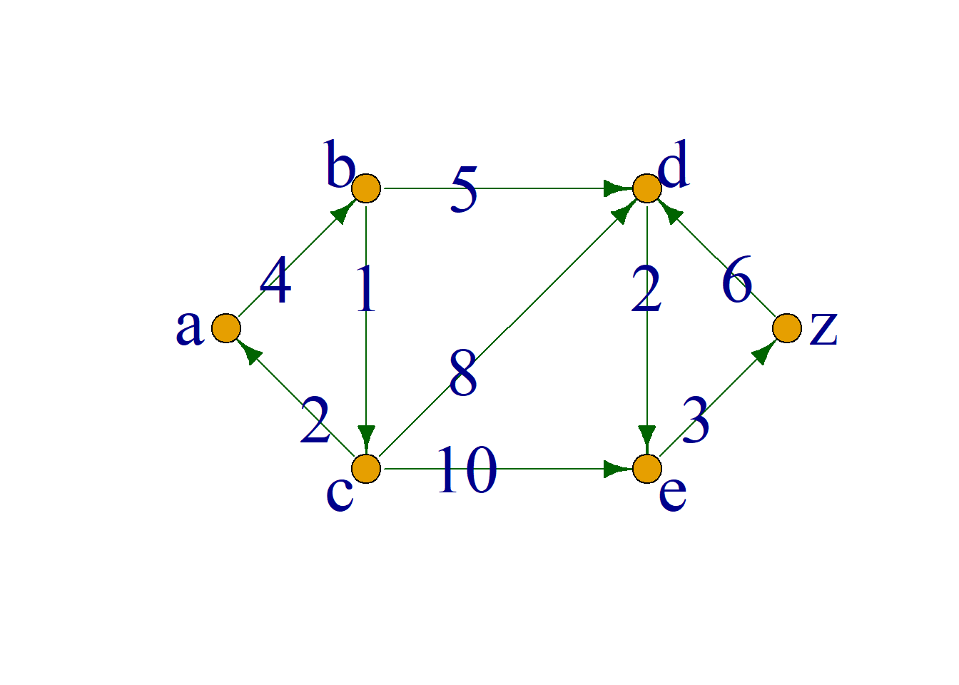
The length of the shortest path between vertices \(v_i\) and \(v_j\) is called the distance from \(v_i\) to \(v_j\), denoted by \(d[v_i, v_j]\).
In practical applications, it is often necessary to find a certain type of subgraph with minimum weight, that is, to find the shortest path between two given nodes, which is the so-called shortest path problem.
Obviously the shortest path between two nodes must be a simple path.
In graph-theoretic terms, the CPP asks for a closed walk in a connected weighted graph \(G={\langle}V, E{\rangle}\) that traverses every edge of \(G\) at least once and has minimum total weight.
That is to say, we need to find a circuit with the smallest weight from the circuit containing each edge of \(G\).
If \(G\) is an Eulerian graph, it is easy to find an Euler circuit by Fleury’s algorithm. However, if \(G\) is not an Eulerian graph, that is, there are vertices of odd degree, and the required loop must pass through certain edges repeatedly, then the solution of the Chinese Postman Problem will be much more difficult.
There are effective solutions to this problem, and one of the most intuitive methods is to copy some edges in the graph into two edges, and then find an Eulerian circuit in the graph you want, that is, the Edmonds-Johnson algorithm:
1 If \(G\) does not contain odd-degree nodes, then any Euler circuit is the solution to the problem.
2 If there are \(2k(k>0)\) vertices of odd degree, first find the shortest path between each pair of them, and then select \(k\) paths \(p_1, p_2, {\cdots}, p_k\) so that the following conditions are met:
Any \(p_i\) and \(p_j (i{\neq}j)\) do not have the same starting point and end point;
Among all the sets of \(k\) shortest paths that satisfy (1), the total length of \(p_1, p_2, {\cdots}, p_k\) is the shortest.
3 According to the \(k\) shortest paths \(p_1, p_2, {\cdots}, p_k\) obtained in 2, copy all the edges that appear on this path in the original graph \(G\), and let the resulting graph be \(G^\prime\).
4 Construct the Euler circuit of \(G^\prime\), and obtain the solution to the Chinese Postman Problem.
Example: As shown in the figure, find a solution to the Chinese Postman Problem.
Solution:
1 Because \(G\) contains nodes of odd degree. Therefore:
2 There are \(2k=4(k=2)\) odd degree nodes \(v_1, v_2, v_3, v_5\) in \(G\). The distance between these 4 points is: \[d[v_1, v_2]=3, d[v_1, v_3]=5, d[v_1, v_5]=4, \] \[d[v_2, v_3]=2, d[v_2, v_5]=3, d[v_3, v_5]=4.\]
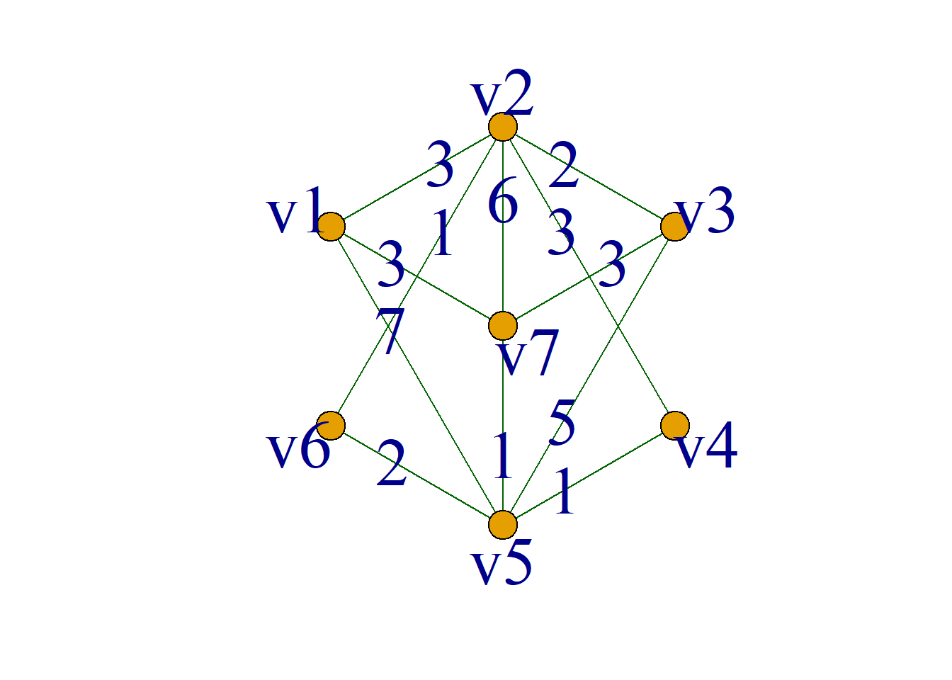
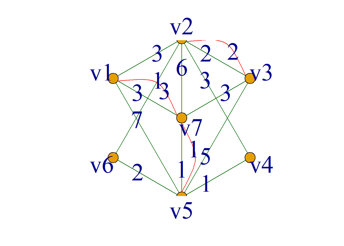
Each path: \[v_1v_2(3), v_3v_5(4){\longmapsto}7\] \[v_1v_3(5), v_2v_5(3){\longmapsto}8\] \[v_1v_5(4), v_2v_3(2){\longmapsto}6\] So the two are the shortest: \(p_1=v_1v_7v_5, p_2=v_2v_3\)
\[p_1=v_1v_7v_5, p_2=v_2v_3.\] Add all the edges on these two paths in \(G\) to get \(G^\prime\).
3 Constructing any Eulerian circuit of \(G^\prime\) is the solution to the Chinese Postman Problem.
Shortest Path Problem
In practical applications, it is often necessary to find a certain type of subgraph with minimum weight, which is the so-called shortest path problem. In 1959, the Dutch mathematician and computer scientist Dijkstra (Dijkstra) proposed an algorithm for finding the shortest path between any two nodes in a weighted graph: Dijkstra’s algorithm.
Dijkstra’s algorithm:
\(L\) represents the current minimum value of the length of the path from node \(u\) to each node, and \(S\) represents the set of nodes for which the shortest path has been obtained.
Initialization. Let \(u=v_1\), \(L(u)=0\), \(L(v_i)=\infty(i=2, 3\cdots, n)\), \(S=\phi\);
If \(|S|=n\), go to (5);
Select \(v\) with the minimum value \(L(v)\) from \(V-S\), let \(S=S\cup\{v\}\);
For all \(x{\in}V-S\), let \(L(x)=\min\{L(x), L(v)+w(v, x)\}\), go to (2);
Output the length of the shortest path \(L(v)\) from \(u\) to each other node.
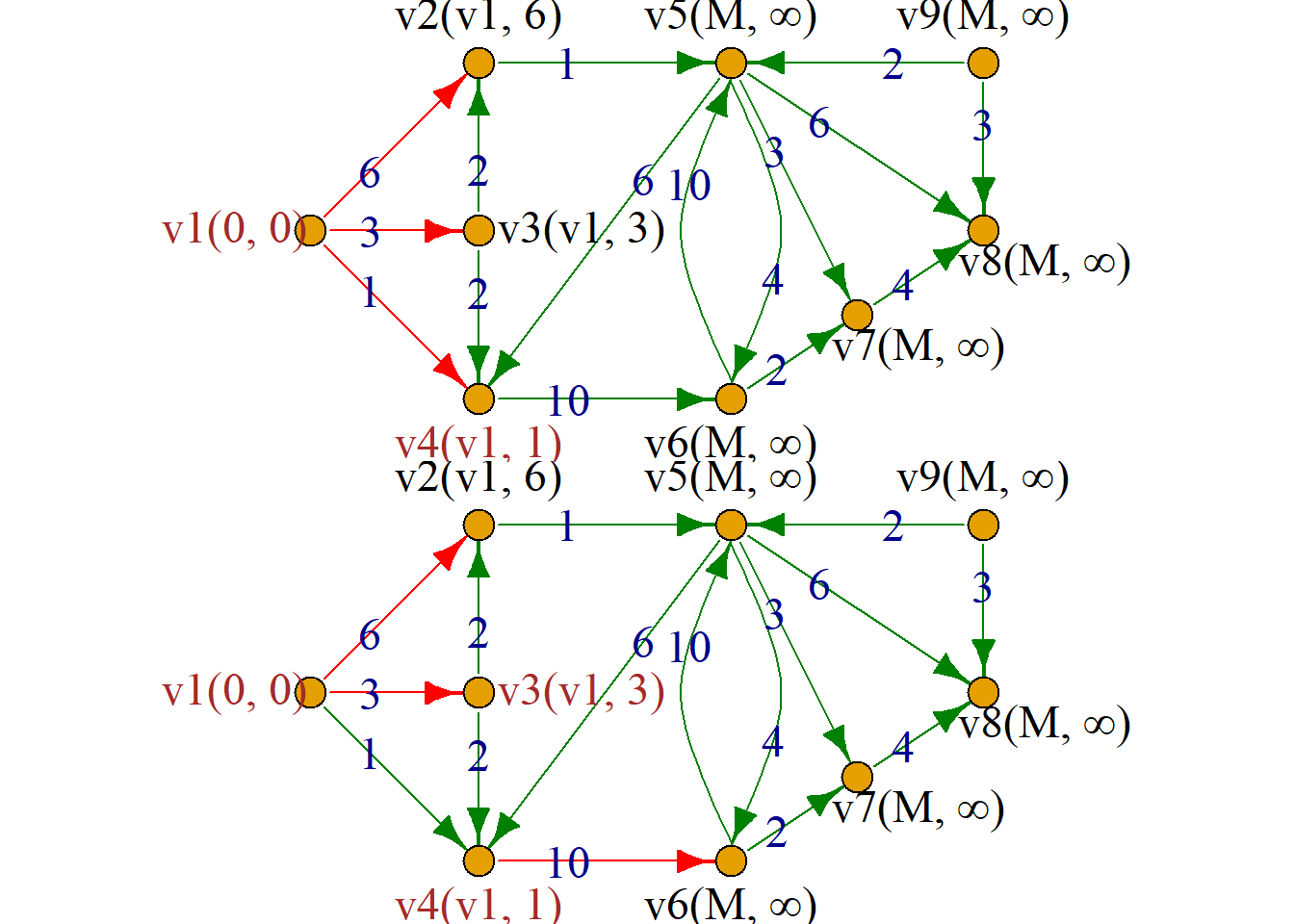
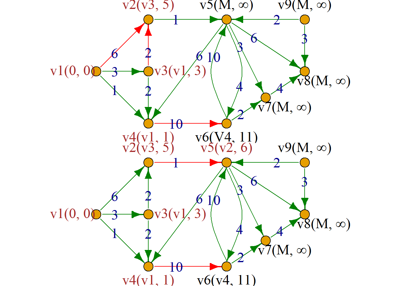
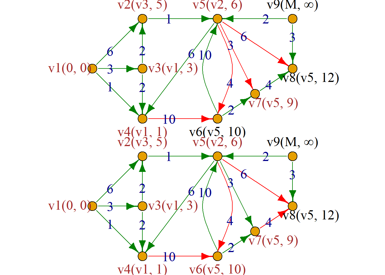
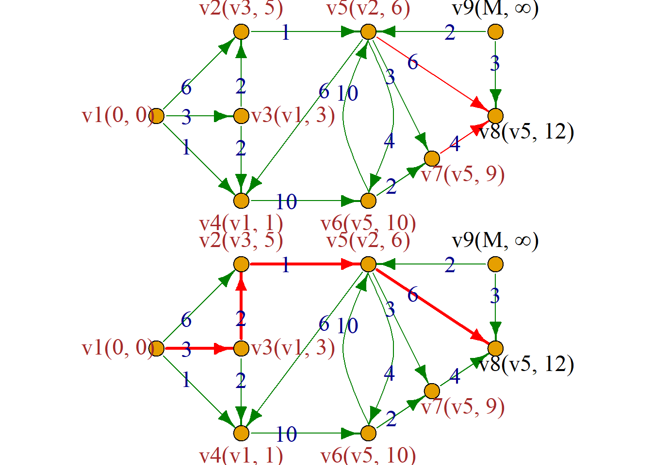
\[ \begin{array}{ccc} Step & Set P & L_1 & L_2 & L_3 & L_4 & L_5 & L_6 & L_7 & L_8 & L_9\\ 0 & \phi & 0 & \infty & \infty & \infty & \infty & \infty & \infty & \infty & \infty\\ 1 & 1 & & 6 & 3 & 1 & \infty & \infty & \infty & \infty & \infty\\ 2 & 14 & & 6 & 3 & & \infty & 11 & \infty & \infty & \infty\\ 3 & 13 & & 5 & & & \infty & 11 & \infty & \infty & \infty\\ 4 & 132 & & & & & 6 & 11 & \infty & \infty & \infty\\ 5 & 1325 & & & & & & 10 & 9 & 12 & \infty\\ 6 & 13257 & & & & & & 10 & & 12 & \infty\\ 7 & 13256 & & & & & & & & 12 & \infty\\ 8 & 13258 & & & & & & & & \\ \end{array} \]
132 represents {\(v1\), \(v3\), \(v2\)}, \(L_1\) represents \(L(v1)\).
Bipartite Graphs
Bipartite graph, also known as bipartite graph (double graph), is a special model in graph theory.
Definition: Given an undirected graph \(G={\langle}V, E{\rangle}\), if the node set \(V\) can be divided into two non-empty subsets \(V_1\) and \(V_2\), satisfying \(V_1{\cup}V_2=V, V_1{\cap}V_2=\phi\), and for any edge \((v_i, v_j)\) in \(G\), If there are \(v_i{\in}V_1, v_j{\in}V_2\), then \(G\) is said to be a bipartite graph (Bipartite graph), often recorded as \(G={\langle}V_1, E, V_2{\rangle}\), \(V_1\) and \(V_2\) are called complementary node subsets of \(G\).
If each node of \(V_1\) is connected to each node of \(V_2\) by one and only one edge, then \(G\) is said to be a complete bipartite graph, often recorded as \(k_{m, n}\), where \(m=|V_1|\), \(n=|V_2|\).
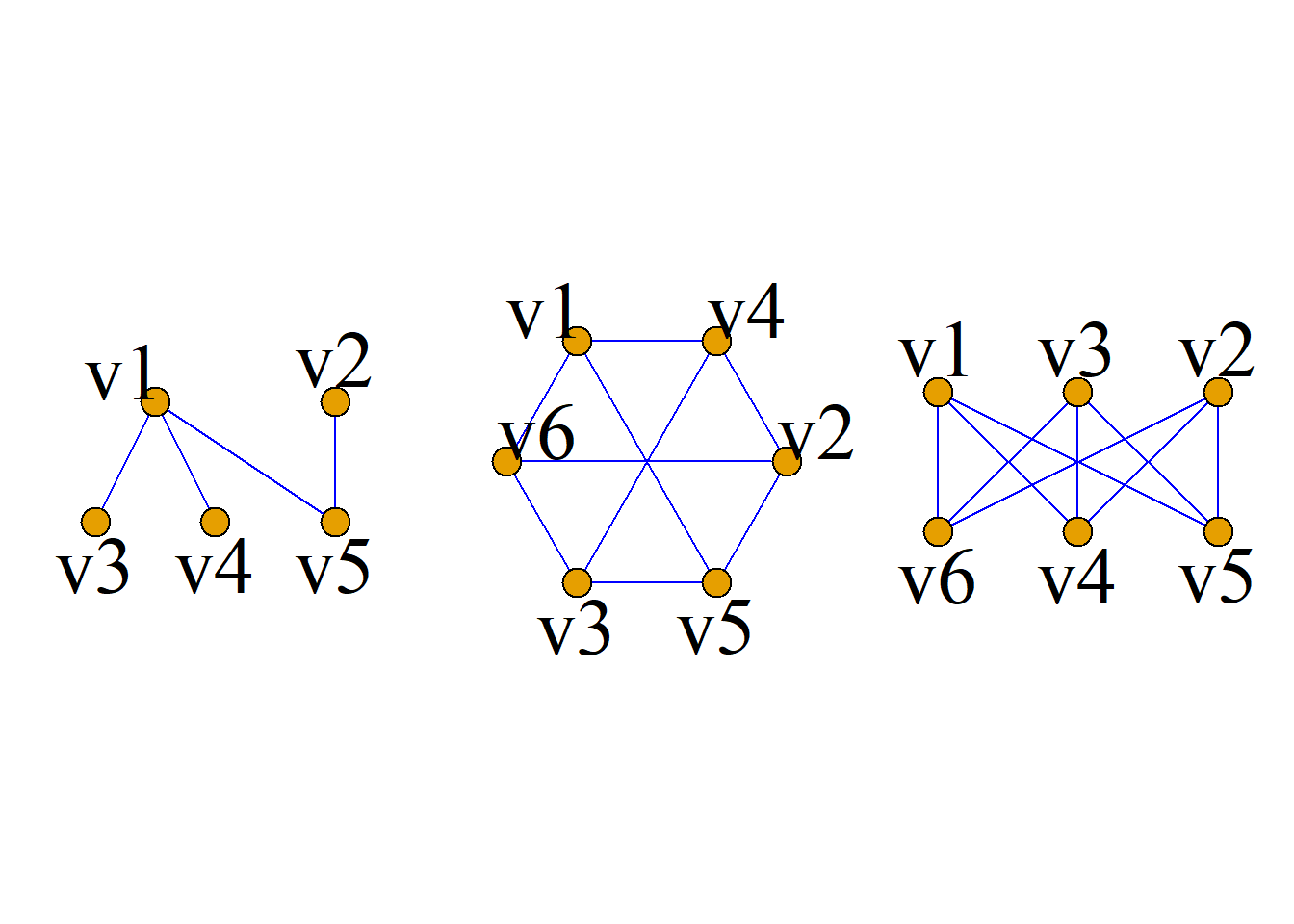
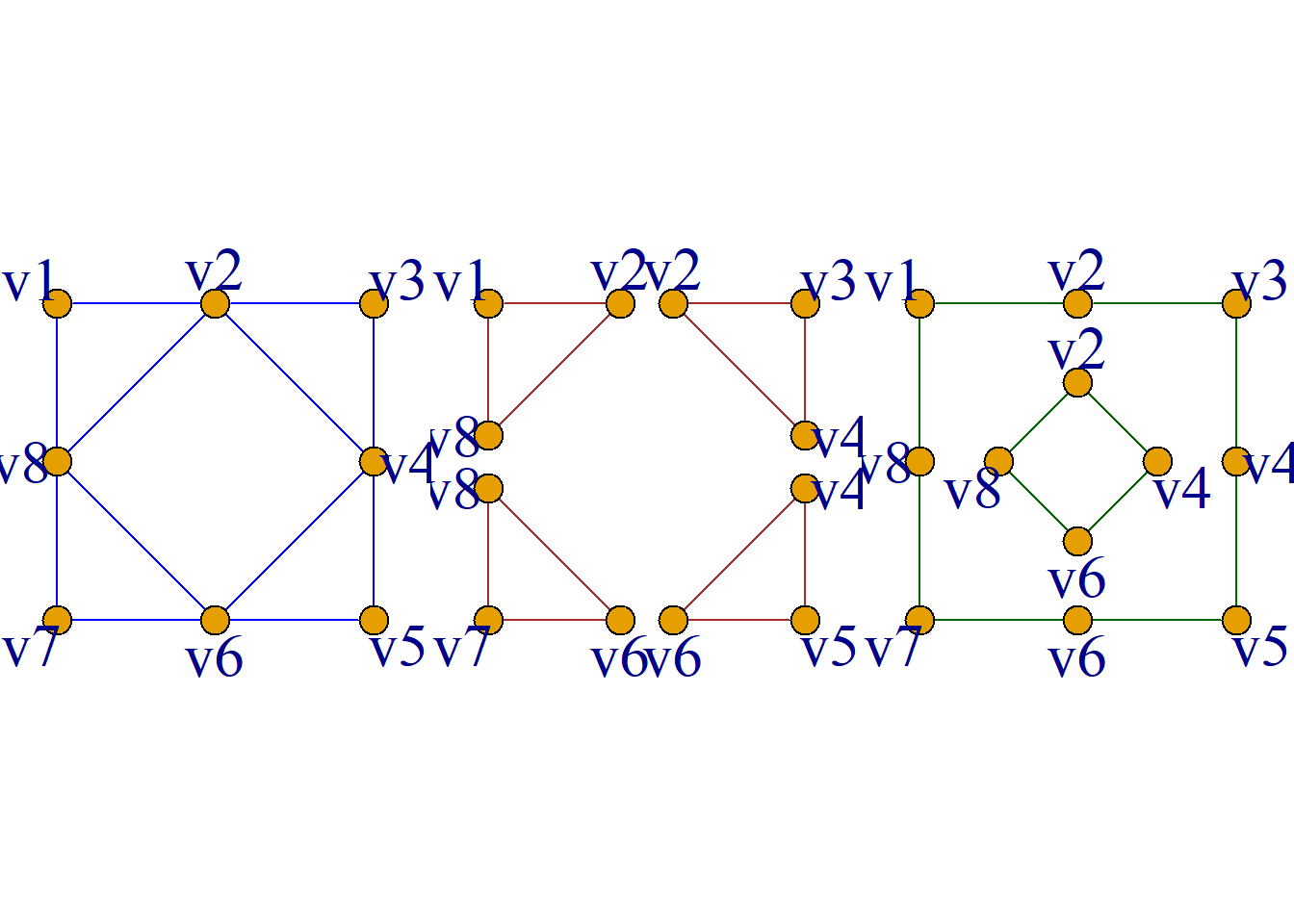
Theorem: The undirected graph \(G={\langle}V, E{\rangle}\) is a bipartite graph if and only if \(G\) has at least two nodes, and the lengths of all loops are even numbers.
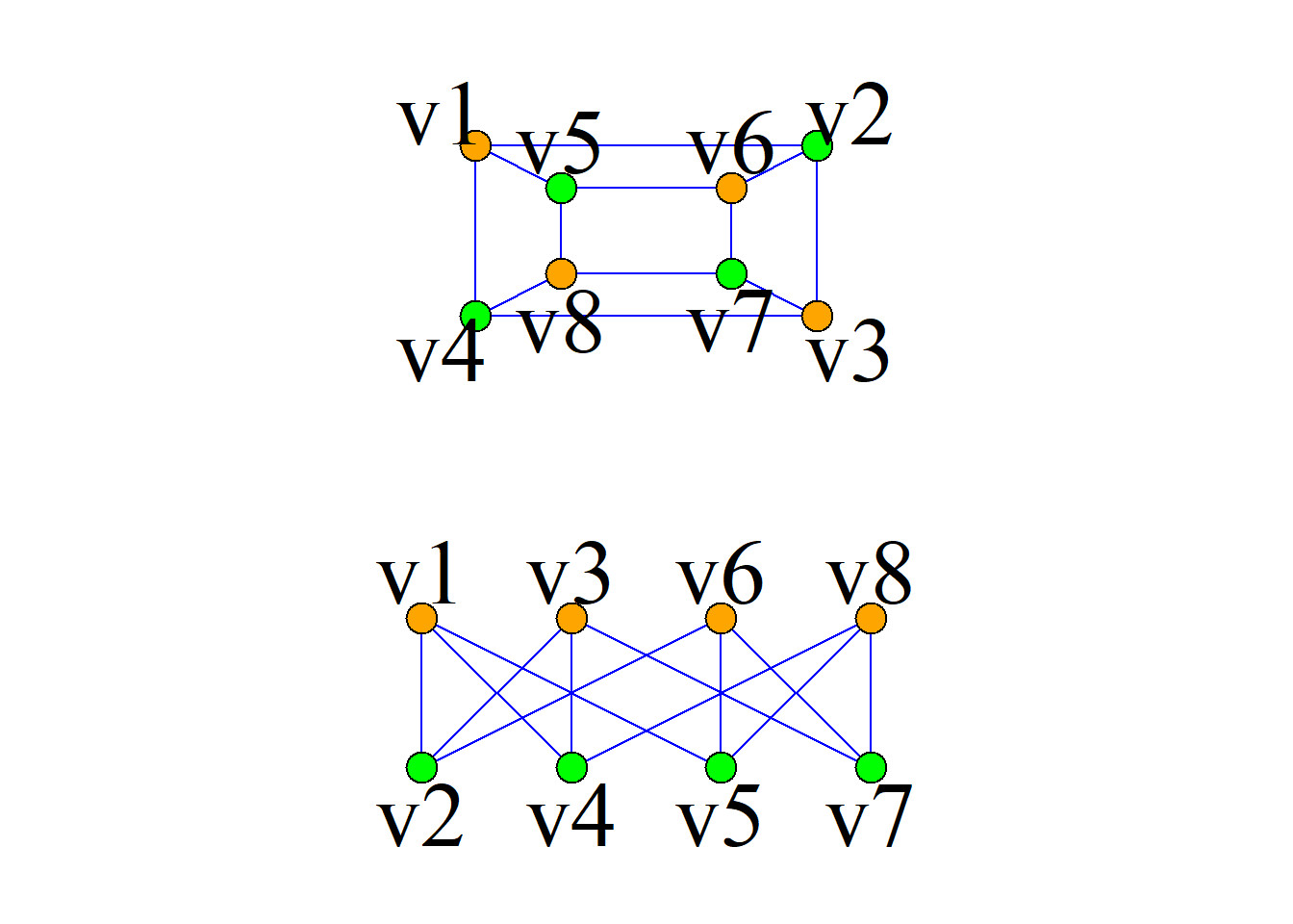
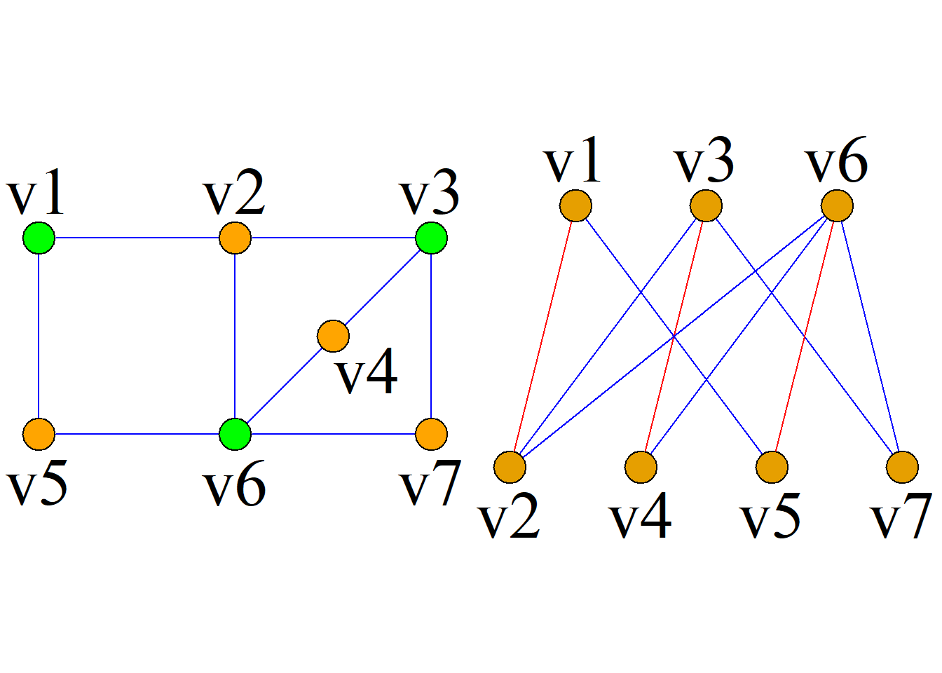
Example: As shown in the figure, is the graph \(G\) a bipartite graph?
Solution: \(G\) is a bipartite graph because all loops in the graph have even lengths.
\[V_1=\{v_1, v_3, v_6, v_8\}\] \[V_2=\{v_2, v_4, v_5, v_7\}\]
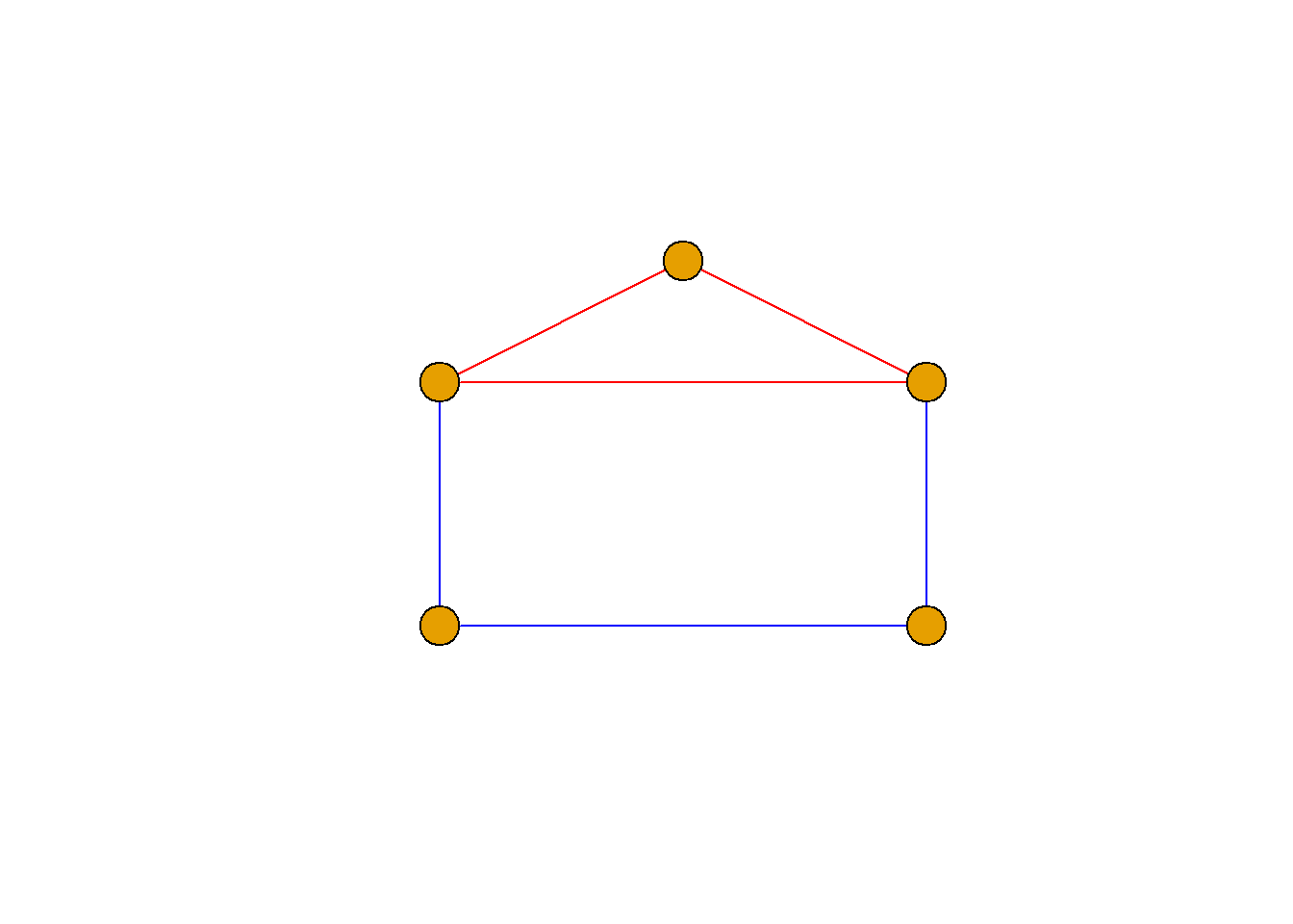
Example: As shown in the figure, is \(G\) a bipartite graph?
Solution: \(G\) is not a bipartite graph because there are cycles with odd lengths in the graph.
Example: A ferryman wants to cross a wolf, a sheep, and a vegetable from the west of the river to the east of the river. Since the boat is small, he can only carry one thing across the river at a time, and the wolf, the sheep, and the sheep and the vegetables cannot be alone, so he gives a plan for crossing the river.
Solution: Use a four-dimensional 0-1 vector to represent the status of humans, wolves, sheep and vegetables on the west coast. If they are on the west coast, the corresponding component takes 1, otherwise it takes 0. A total of \(2^4=16\) states: (0, 0, 0, 0), (0, 0, 0, 1), (0, 0, 1, 0), \({\cdots}\), (1, 1, 1, 0), (1, 1, 1, 1)
16 states (human, wolf, sheep, vegetable): (0, 0, 0, 0), (0, 0, 0, 1), (0, 0, 1, 0), \({\cdots}\), (1, 1, 1, 0), (1, 1, 1, 1).
According to the question, the states (0, 1, 1, 0), (0, 0, 1, 1), (0, 1, 1, 1) are not allowed; The opposite states (1, 0, 0, 1), (1, 1, 0, 0), (1, 0, 0, 0) are also not allowed.
Allowed states: (1, 1, 1, 1), (1, 1, 1, 0), (1, 1, 0, 1), (1, 0, 1, 1), (1, 0, 1, 0), (0, 1, 0, 1), (0, 0, 0, 1), (0, 0, 1, 0), (0, 1, 0, 0), (0, 0, 0, 0).
Question: How to move from state (1, 1, 1, 1) to (0, 0, 0, 0)?
Allowed state vectors:
People in the West Bank: (1, 1, 1, 1), (1, 1, 1, 0), (1, 1, 0, 1), (1, 0, 1, 1), (1, 0, 1, 0)
People on the east coast: (0, 1, 0, 1), (0, 0, 0, 1), (0, 0, 1, 0), (0, 1, 0, 0), (0, 0, 0, 0)
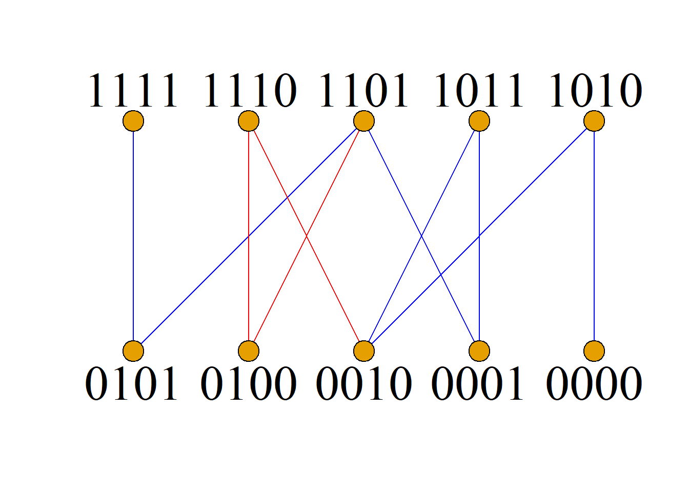
Record the 10 nodes as \(A_1, A_2, {\cdots}, A_{5}\) (top row from left to right), \(A_6, A_7, {\cdots}, A_{10}\) (bottom row from left to right).
Can the river-crossing problem be solved? That is, are \(A_1\) to \(A_{10}\) in the picture connected? How many different solutions are there? That is, how many different paths are there from \(A_1\) to \(A_{10}\)? What’s the fastest solution? That is, which is the shortest path from \(A_1\) to \(A_{10}\)?
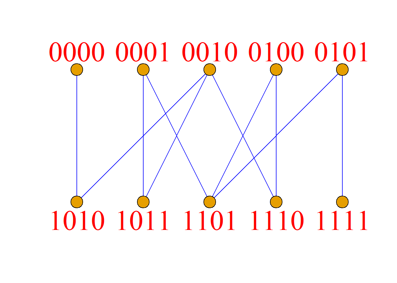
Method: Start from \((1, 1, 1, 1)\), go along the associated edges to reach the unreached adjacent points, and end at \((0, 0, 0, 0)\) to get the directed graph.
Two paths can be obtained from the figure:
\[A_1A_6A_3A_7A_2A_8A_5A_{10}\] \[A_1A_6A_3A_9A_4A_8A_5A_{10}\]
The farmer leads the sheep across the river; The farmer returns; The farmer leads the wolf across the river; The farmer returns with his sheep; The farmer carries vegetables across the river; The farmer returns; The farmer leads the sheep across the river.
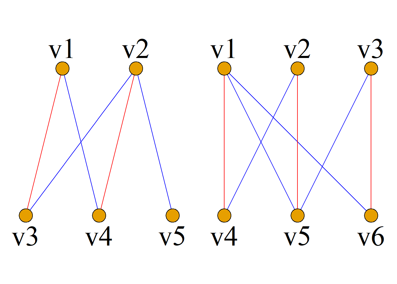
Definition: Let \(G={\langle}V_1, E, V_2{\rangle}\) be a bipartite graph. If \(M{\subseteq}E\) and no two edges in \(M\) are adjacent, then \(M\) is called a matching of \(G\). A matching with the largest number of edges is called a maximum matching.
If every vertex in \(V_1\) is incident to an edge in \(M\), then \(M\) is called a \(V_1\)-complete matching. If every vertex in \(V_2\) is incident to an edge in \(M\), then \(M\) is called a \(V_2\)-complete matching.
If \(M\) is both a \(V_1\)-complete matching and a \(V_2\)-complete matching, then \(M\) is called a perfect matching of \(G\).
\(V_1\)-complete matching, \(V_2\)-complete matching, and perfect matching are all maximum matchings, but the converse is not true.
A maximum matching always exists, but it is not necessarily unique.
Example: In (a), {\((v_1, v_3)\), \((v_2, v_4)\)} is a \(V_1\)-complete matching, and it is also a maximum matching;
In (b), {\((v_1, v_4)\), \((v_2, v_5)\), \((v_3, v_6)\)} is both a \(V_1\)-complete matching and a \(V_2\)-complete matching, so it is a perfect matching.
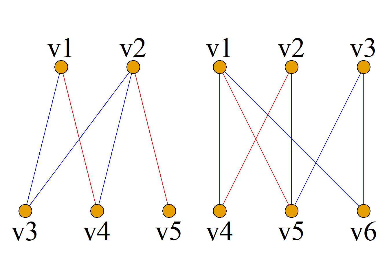
A matching is not necessarily unique: As shown in (a), {\((v_1, v_4)\), \((v_2, v_5)\)} is a \(V_1\)-complete matching, and it is also a maximum matching;
In (b), {\((v_1, v_5)\), \((v_2, v_4)\), \((v_3, v_6)\)} is both a \(V_1\)-complete matching and a \(V_2\)-complete matching, so it is a perfect matching.
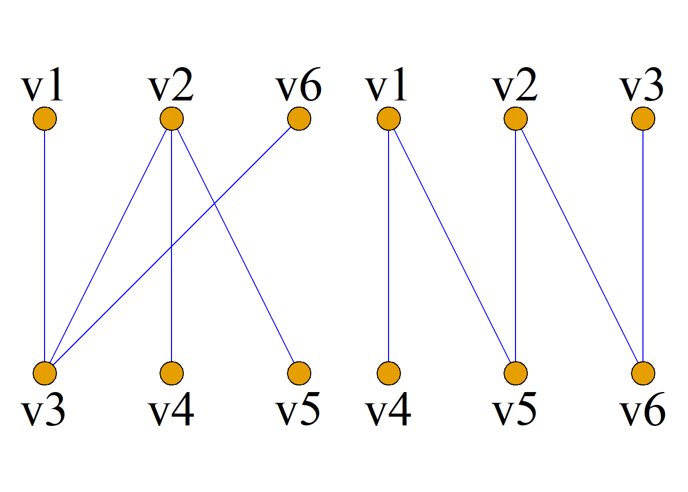
Theorem: Hall’s Marriage Theorem Let \(G={\langle}V_1, E, V_2{\rangle}\) be a bipartite graph. A necessary and sufficient condition for the existence of a \(V_1\)-complete matching is: For any \(S{\subseteq}V_1\) we have \[|N(S)|{\geq}|S|\] where \(|N(S)|\) is the size of the neighborhood of \(S\) (the set of vertices adjacent to vertices in \(S\)).
(Or: Let \(G={\langle}V_1, E, V_2{\rangle}\) be a bipartite graph, \(G\) has \(V_1\)-complete matching if and only if any \(k\) nodes in \(V_1\) are adjacent to at least \(k\) nodes in \(V_2\), \(k=1, 2, 3\), \({\cdots}\), \(|V_1|\), \(|V_1|{\leq}|V_2|\).) This condition is called the “dissimilarity condition”.
As shown in the figure, there is no \(V_1\)-complete matching in \(G_1\), and \(V_1\)-complete matching exists in \(G_2\).
Prove: If the bipartite graph \(G={\langle}V_1, E, V_2{\rangle}\) is a \(k\)-regular graph, then there is a complete matching in \(G\).
Proof: Since \(G={\langle}V_1, E, V_2{\rangle}\) is a \(k\)-regular graph, we have \[k{\cdot}|V_1|=|E|=k{\cdot}|V_2|\] Thus we get \(|V_1|=|V_2|\).
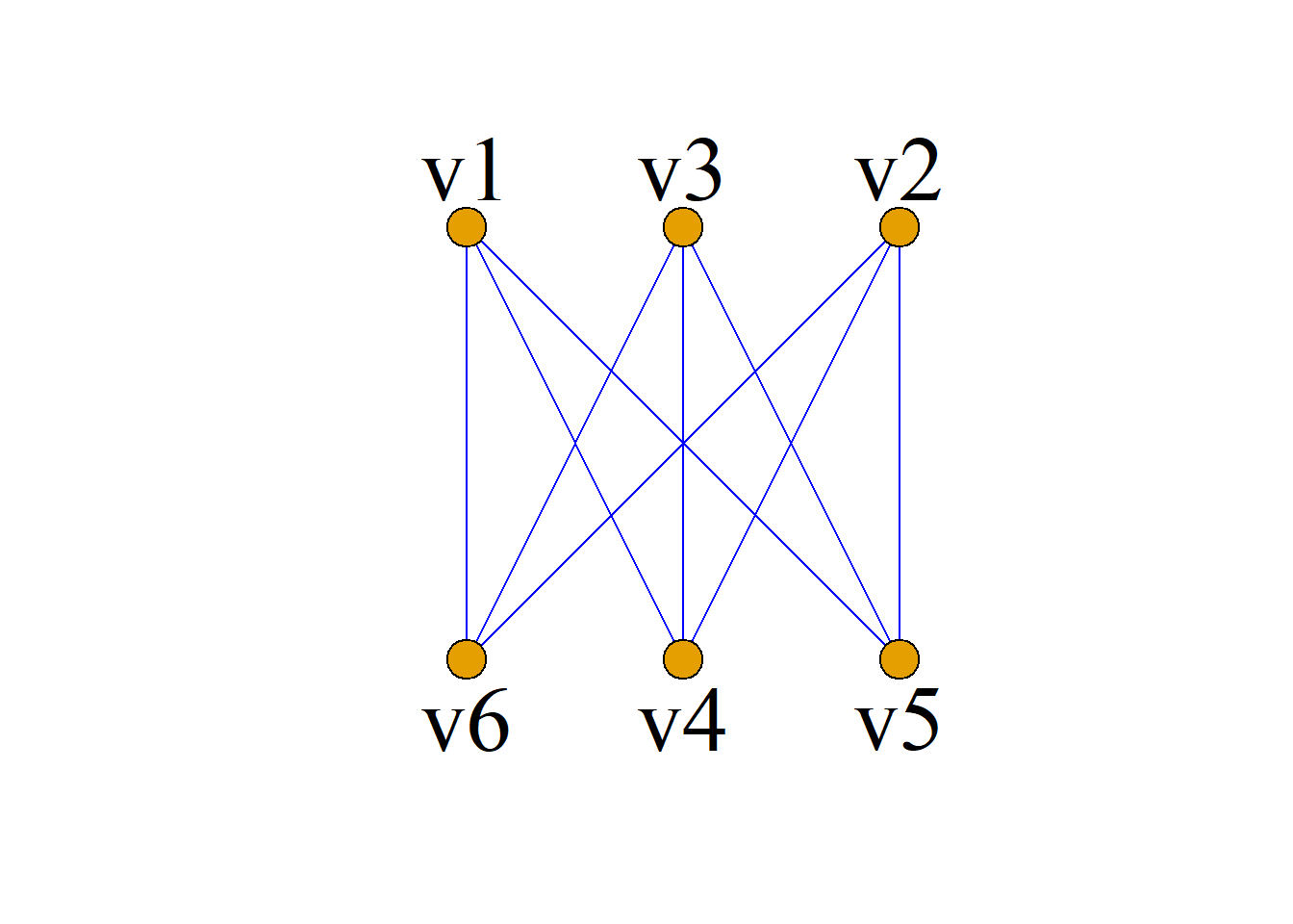
Let any \(S{\subseteq}V_1, N(S)\) be the set of adjacent nodes of \(S\), \(E_1\) be the set of edges associated with the nodes in \(S\), \(E_2\) be the set of edges associated with the nodes in \(N(S)\), it can be seen that \(E_1{\subseteq}E_2\), then \[k{\cdot}|N(S)|=|E_2|{\geq}|E_1|=k{\cdot}|S|\] We get \(|N(S)|{\geq}|S|\), so \(G\) has \(V_1\) - exactly matching \(M\).
And since \(|V_1|=|V_2|\), obviously \(M\) is also a complete matching of \(V_2\), so \(M\) is a complete matching of \(G\), that is, there is a complete matching in \(G\).
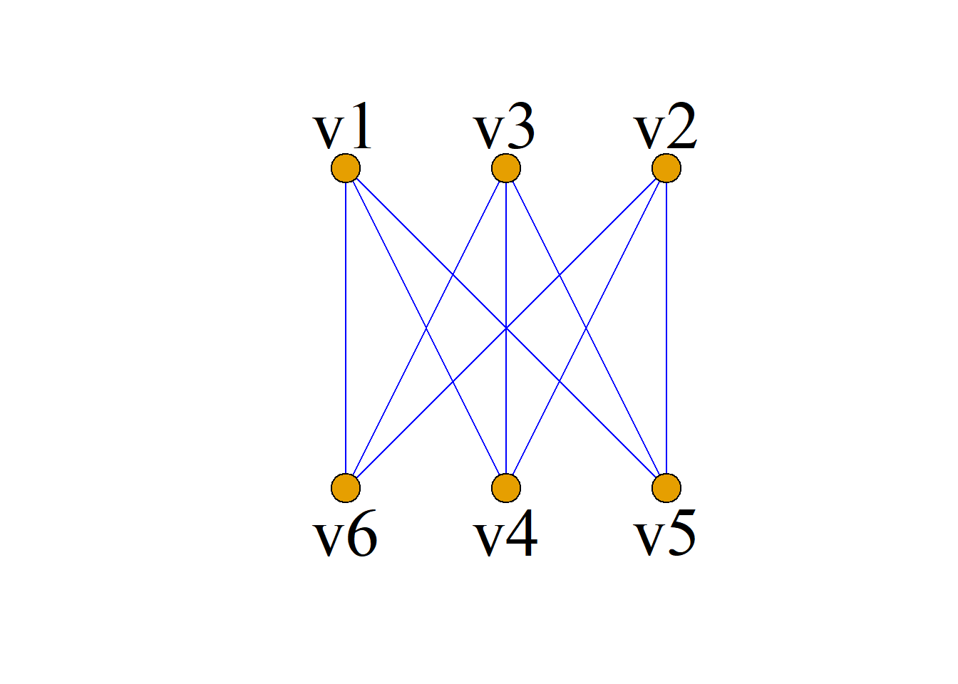
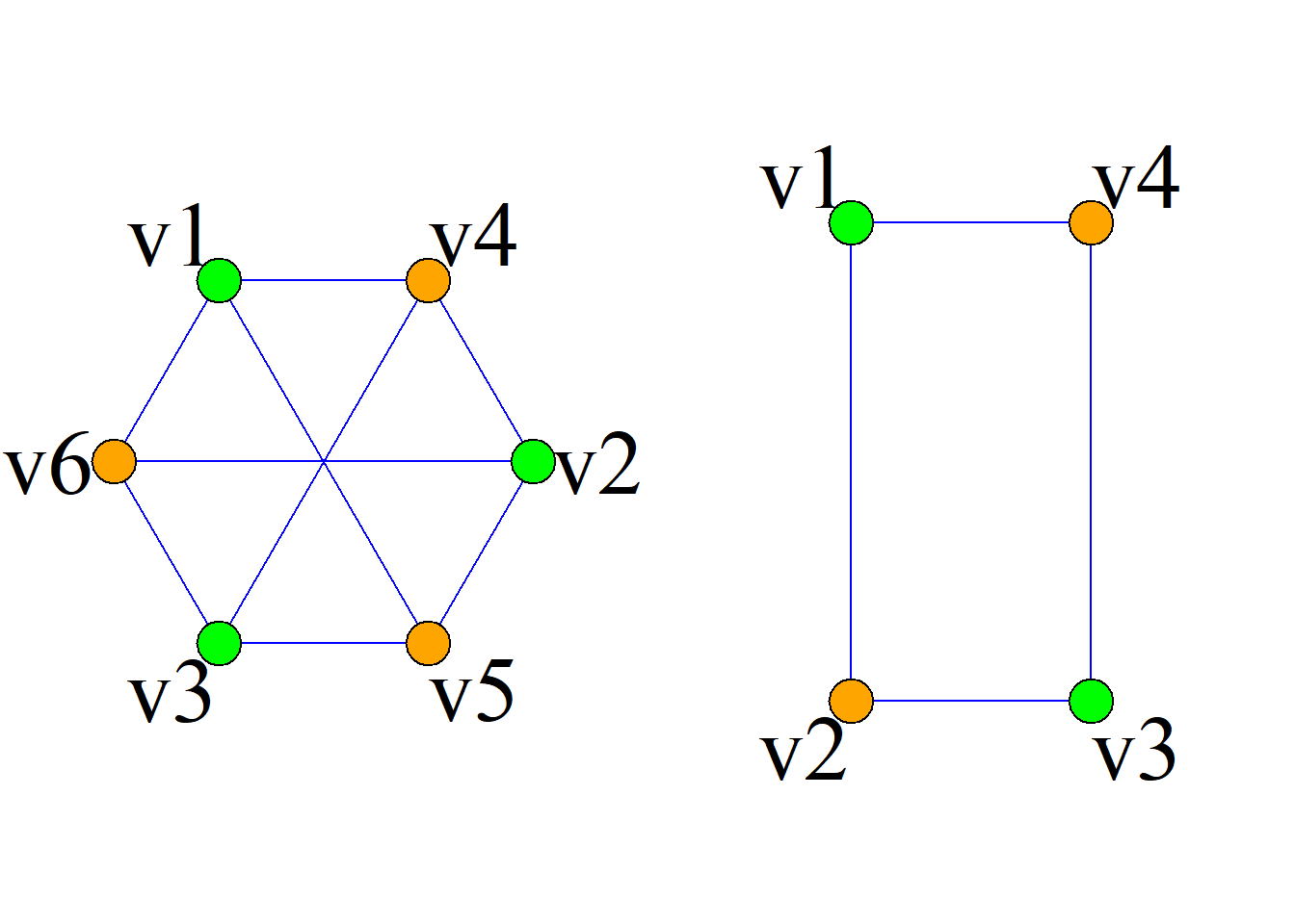
\(G_1\) is a 3-regular graph, then there is a complete matching in \(G_1\);
\(G_2\) is a 2-regular graph, then there is a complete matching in \(G_2\).
Theorem: (\(t\) condition) Suppose \(G={\langle}V_1, E, V_2{\rangle}\) is a bipartite graph. If there is a positive integer \(t\), it satisfies:
For each node in \(V_1\), there are at least \(t\) edges associated with it;
For each node in \(V_2\), there are at most \(t\) edges associated with it.
Then there must be a complete matching of \(V_1\) in \(G\).
That is: the minimum value of the node degree in \(V_1\) is greater than or equal to the maximum value of the node degree in \(V_2\). The \(t\) condition is a sufficient condition, but not a necessary condition.
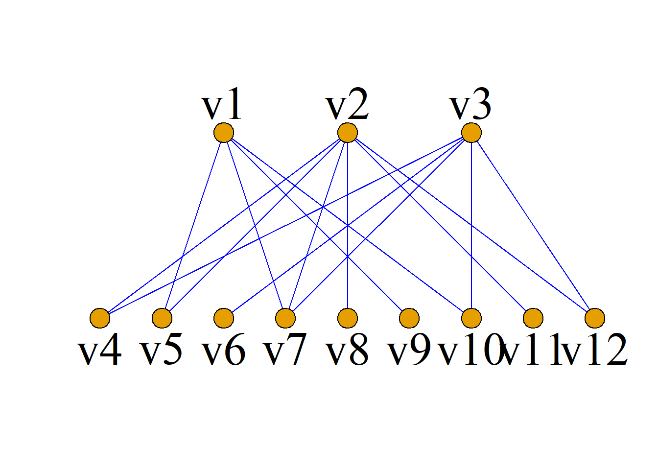
Determine whether there is a \(V_1\)-complete matching in the following bipartite graph? Among them, the complementary node subset:
\(V_1=\{v_1, v_2, v_3\}\),
\(V_2=\{v_4, v_5, v_6, v_7, v_8, v_9, v_10, v_{11}, v_{12}\}\).
Solution: Taking \(t=3\), obviously this bipartite graph satisfies the “\(t\) condition”, so there is \(V_1\) in \(G\) - a perfect match.
Example: Determine whether \(G\) in the following figure is a bipartite graph, and whether there is a \(V_1\)-complete matching?
Solution: It is a bipartite graph, a subset of complementary nodes:
\(V_1=\{v_1, v_3, v_6\}\),
\(V_2=\{v_2, v_4, v_5, v_7\}\).
Although this bipartite graph does not satisfy the “\(t\) condition”, there is a complete matching of \(V_1\) in \(G\).
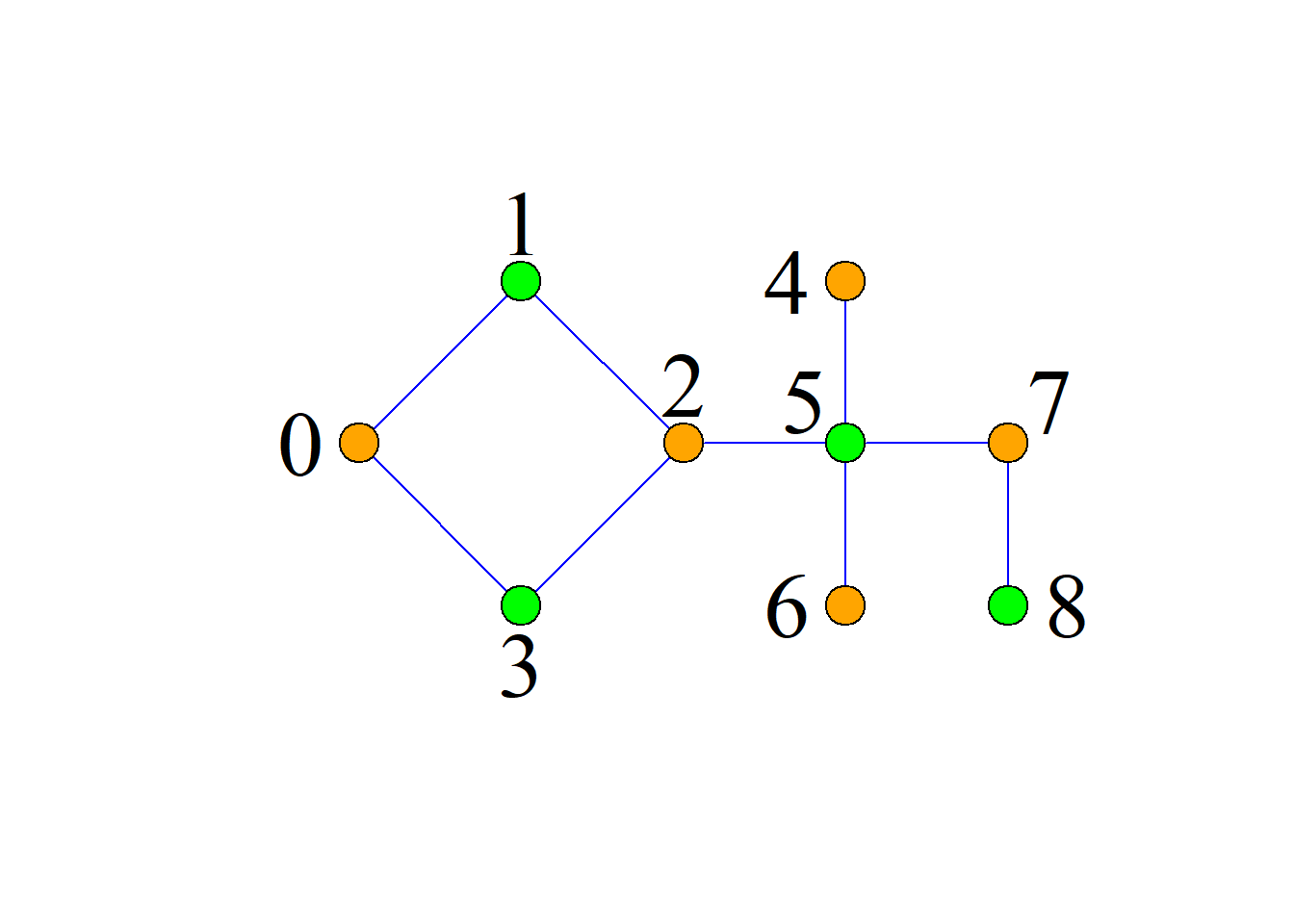
Example: Determine whether the following figure is a bipartite graph and whether there is a complete matching?
Solution: It is a bipartite graph.
Example: Today, four teachers, Li Fang, Guo Qian, Wang Gang and Liu Wei, are assigned to teach four courses: discrete mathematics, data structure, operating system and compilation principles.
It is known that Li Fang is familiar with data structures and operating systems; Guo Qian is familiar with discrete mathematics and compilation principles; Wang Gang is familiar with discrete mathematics, data structures and operating systems; Liu Wei is only familiar with operating systems.
I wonder if a plan can be developed so that everyone can teach the courses they are familiar with and have someone teach each course?
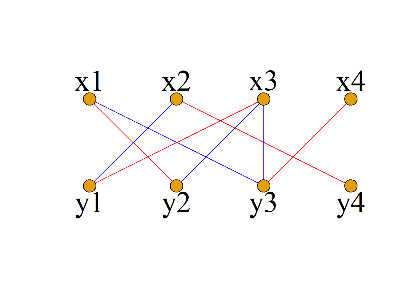
Solution: Let \(x_1, x_2, x_3\) and \(x_4\) represent the four teachers Li Fang, Guo Qian, Wang Gang and Liu Wei respectively, let \(y_1, y_2, y_3\) and \(y_4\) represent the four courses of discrete mathematics, data structure, operating system and compilation principle respectively.
Let \(V_1=\{x_1, x_2, x_3, x_4\}\), \(V_2=\{y_1, y_2, y_3, y_4\}\),
\(E=\{(x_i, y_j)|x_i is familiar with y_j, i, j=1, 2, 3, 4\}\),
Construct an undirected graph \(G={\langle}V, E{\rangle}\). Obviously, this is a bipartite graph, and the original problem is transformed into finding a complete matching in the bipartite graph \(G\).
There is a perfect matching \(\{(x_1, y_2), (x_2, y_4), (x_3, y_1), (x_4, y_3)\}\) in the picture
This perfect matching can be arranged:
Li Fang teaches data structure, Guo Qian teaches compilation principles, Wang Gang teaches discrete mathematics, and Liu Wei teaches operating systems.
Basic concepts of floor plan
The problem of whether the edges of a picture do not cross on a plane is the problem of planarization of the picture. It is widely used in single-sided printed circuit boards, integrated circuit wiring, communications, transportation, urban architecture, etc.
Definition: Suppose \(G={\langle}V, E{\rangle}\) is an undirected graph. If \(G\) can be drawn on a plane, and any two edges have no other intersections except the endpoints, then \(G\) is called a planar graph. This method of drawing the graph is called the planar representation (planar embedding) of the graph. Otherwise, \(G\) is called non-planar graph.
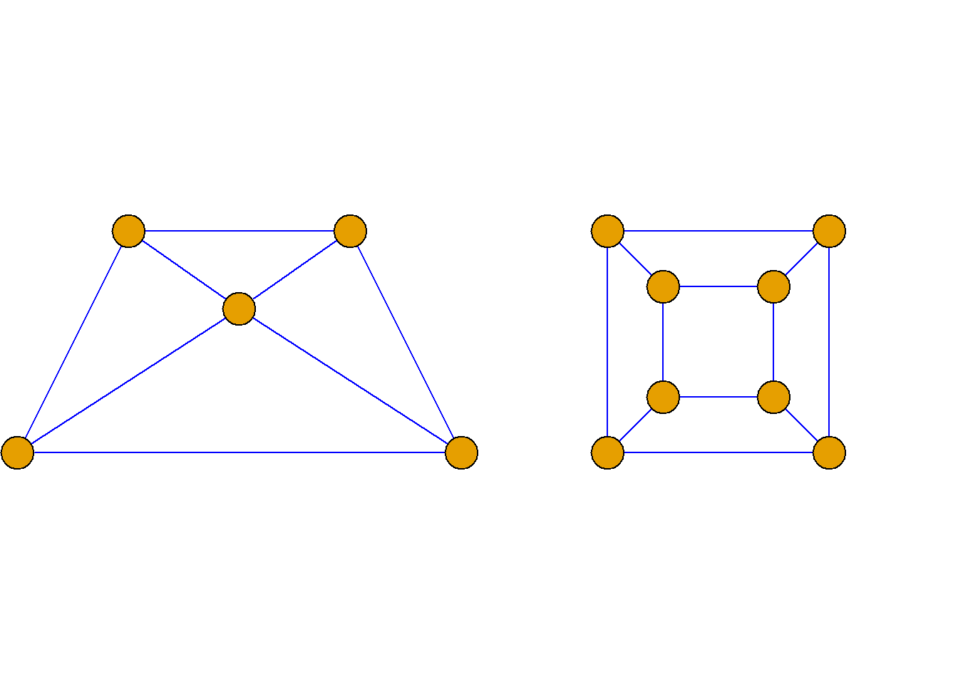
Example: As shown in the figure, (a) is a plan view and (b) is a plan view.
Some graphs cannot be seen from the surface as planar graphs, but they can be transformed into planar graphs through isomorphic transformation. Such graphs are planarizable and are called planar graphs, which are also planar graphs.
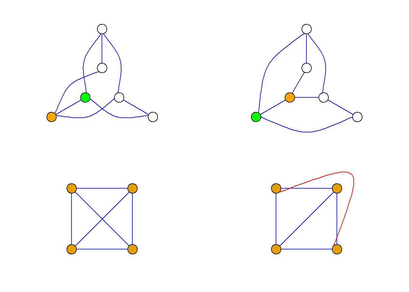
Example: As shown in figure (a), it is a planar graph, and (b) is its planar embedding.
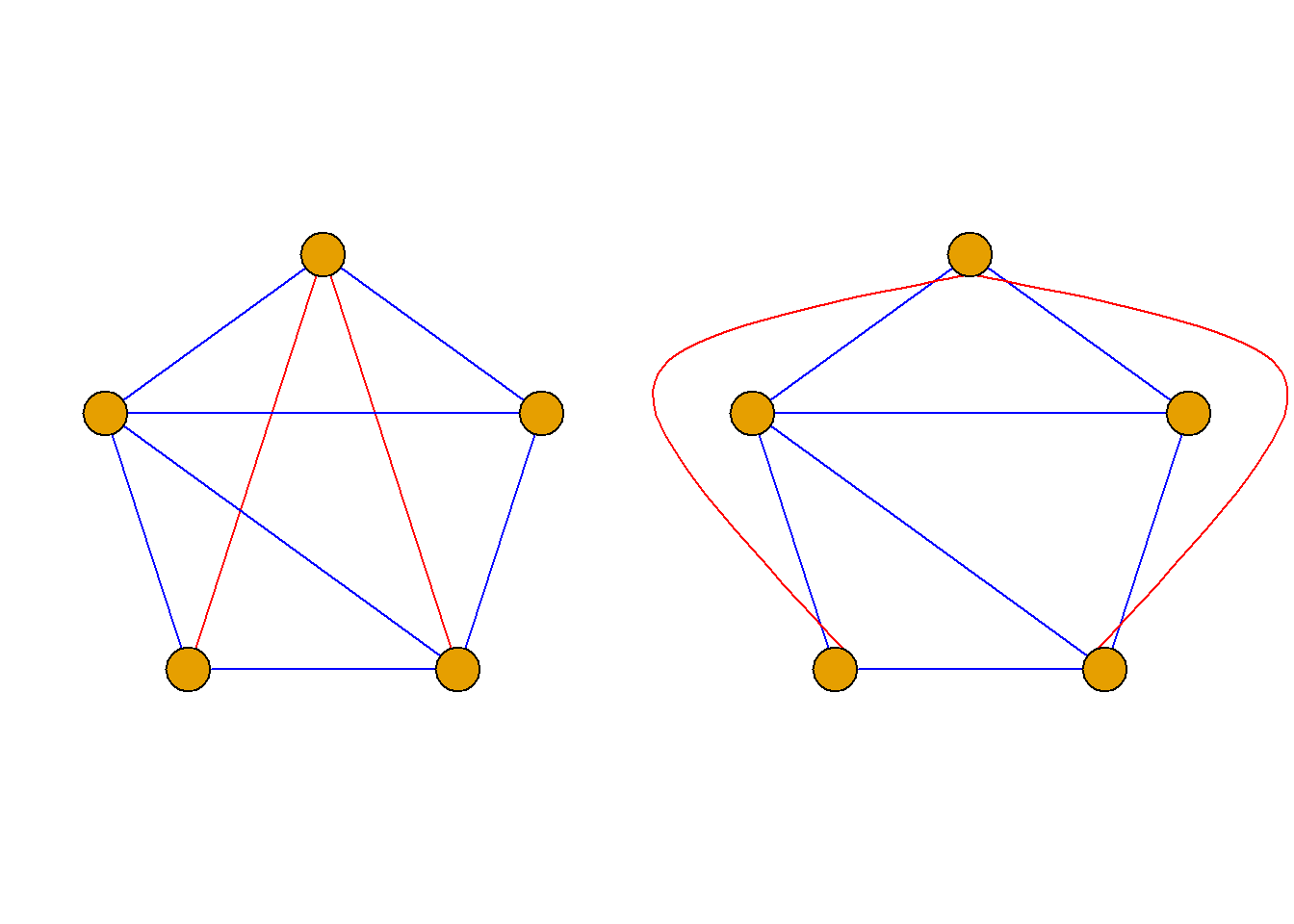
As shown in Figures (1) and (3), it is a plan view.
- is the plane embedding of (1); (4) is the plane embedding of (3).
But some diagrams are not planar diagrams and cannot be flattened.
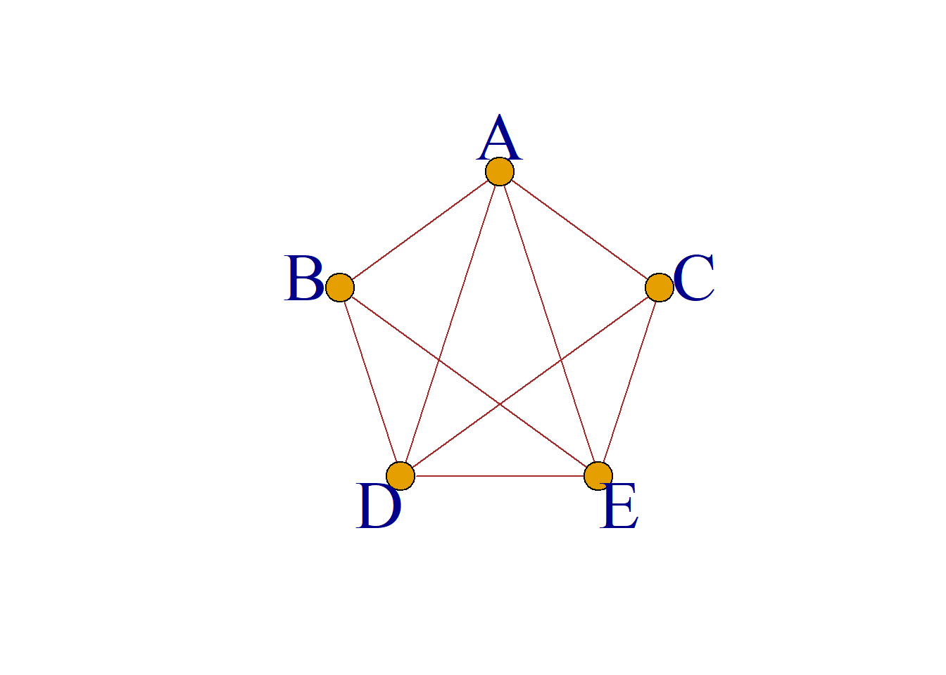
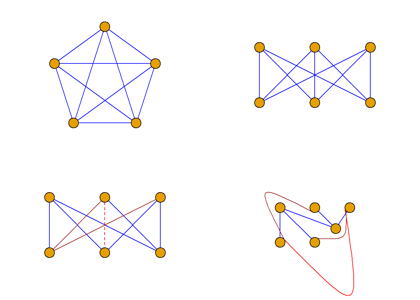
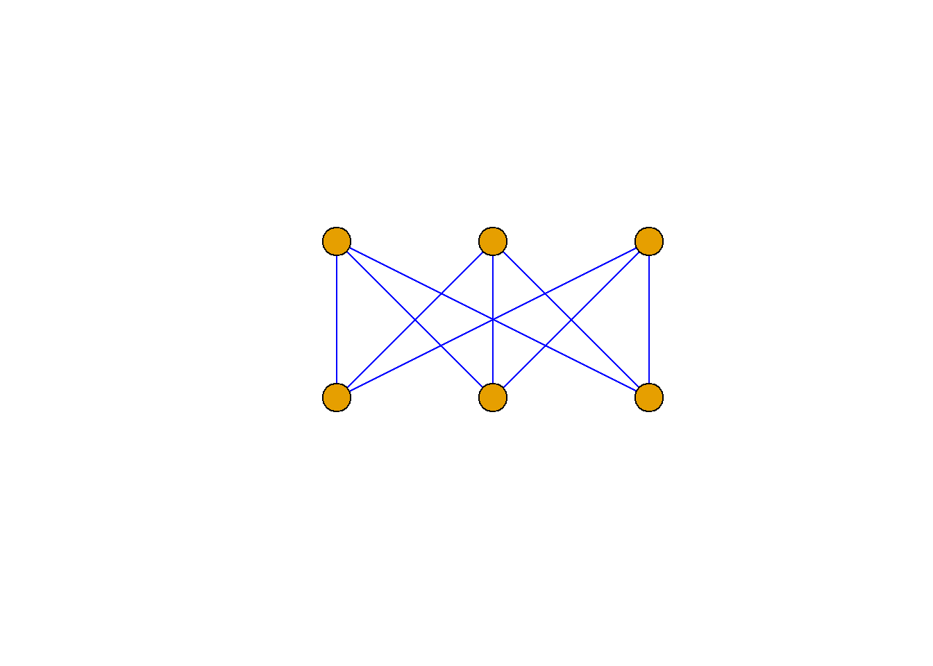
Example: As shown in the figure, \(K_5\) is not a plane diagram; \(K_{3, 3}\) is not a plane diagram either.
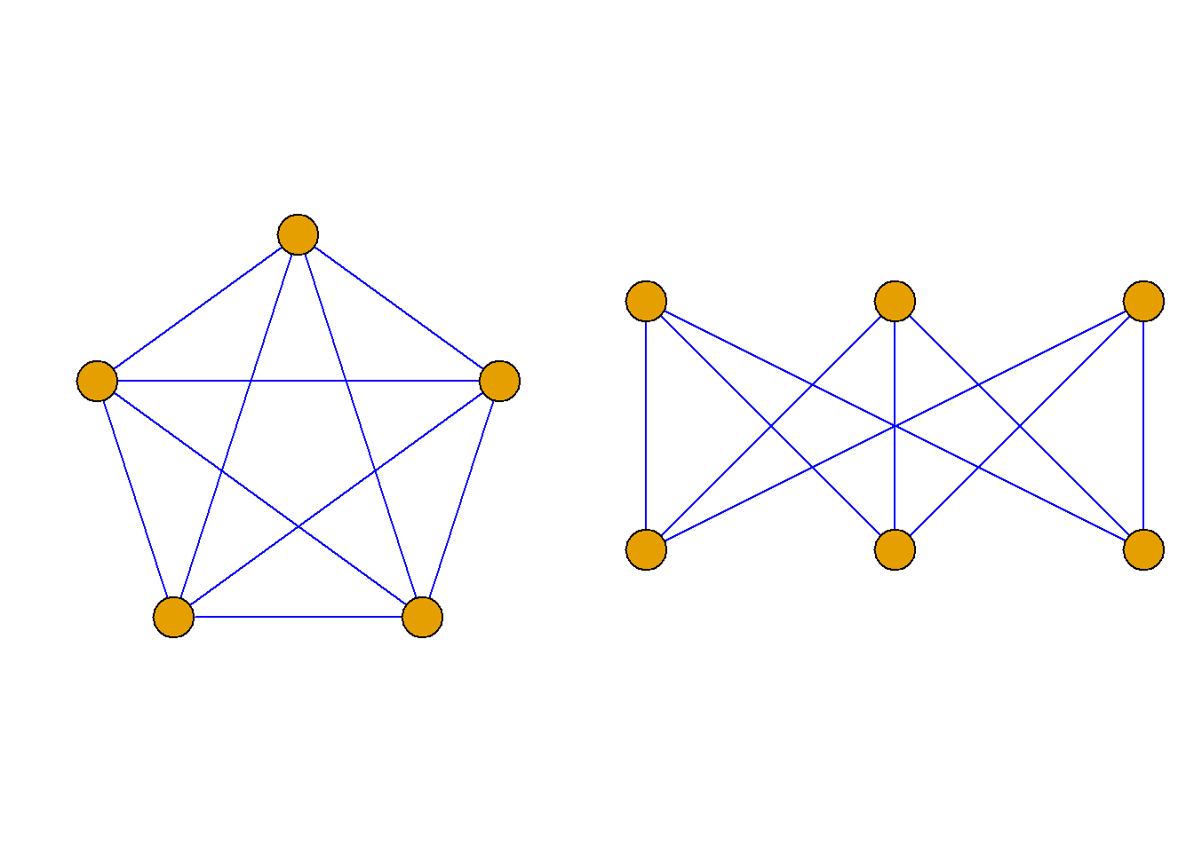
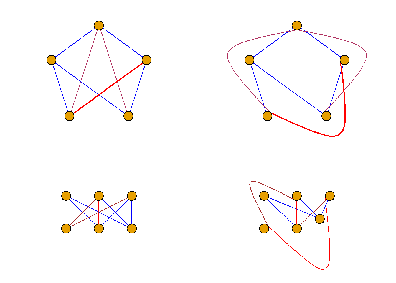
\(k_5\) and \(k_{3, 3}\) are called Kuratowski diagrams, and they have some things in common:
They are both regular graphs (\(k_5\) is a 4-regular graph, \(k_{3, 3}\) is a 3-regular graph);
After removing one side, they are both planar graphs;
\(k_{3, 3}\) is the non-planar graph with the smallest number of edges, and \(k_5\) is the non-planar graph with the smallest number of nodes. They are both the most basic non-planar graphs.
Surface of floor plan
Definition: Suppose \(G\) is a connected plane graph. The edges of \(G\) divide the plane where \(G\) is located into several regions that do not contain nodes and edges. Each region is called a face of \(G\).
The area with limited area is called finite surface or internal surface, and the area with infinite area is called infinite surface or external surface.
The loop formed by all the edges of each face is called the boundary of the face, and its length is called the degree (degree) of the face. The degree of a face f is recorded as \(deg(f)\). If the boundaries of two faces have at least one common edge, they are called adjacent faces.
A connected plane graph is often written as \(G={\langle}V, E, F{\rangle}\), where \(F\) is the set of all faces in the graph.
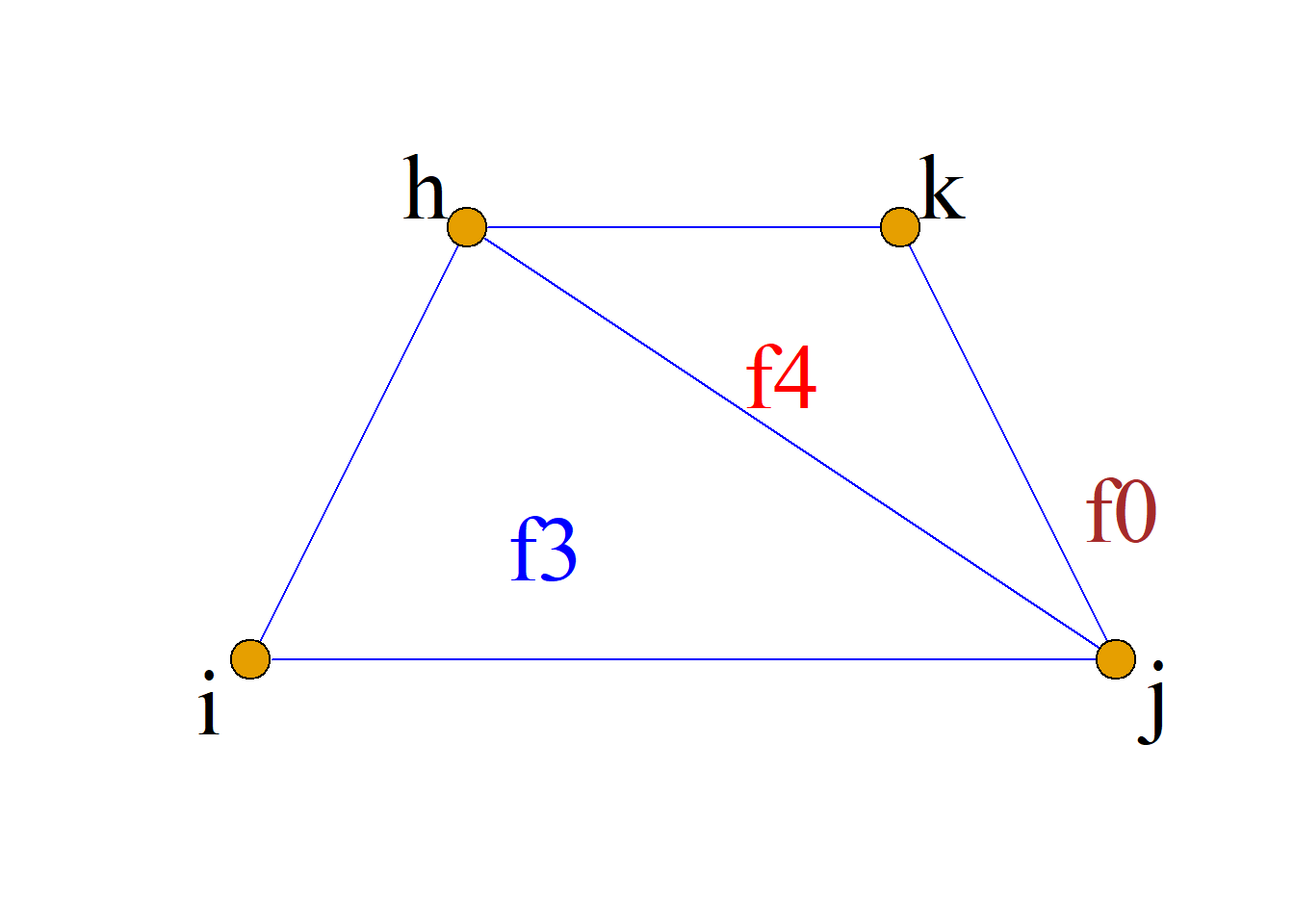
Example: The figure shows a plan view.
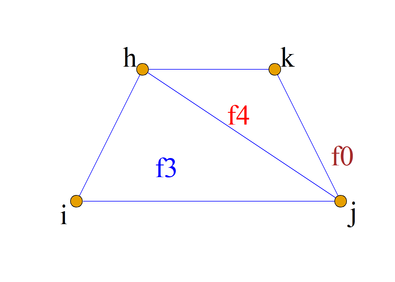
It has a total of 3 faces \(f_3, f_4, f_0\), of which \(f_0\) is an infinite face and the rest are finite faces.
The boundary of \(f_3\) is \((j, h, i, j)\), and the degree is 3;
The boundary of \(f_4\) is \((j, k, h, j)\), and the degree is 3;
The boundary of \(f_0\) is \((j, k, h, i, j)\), and the degree is 4.
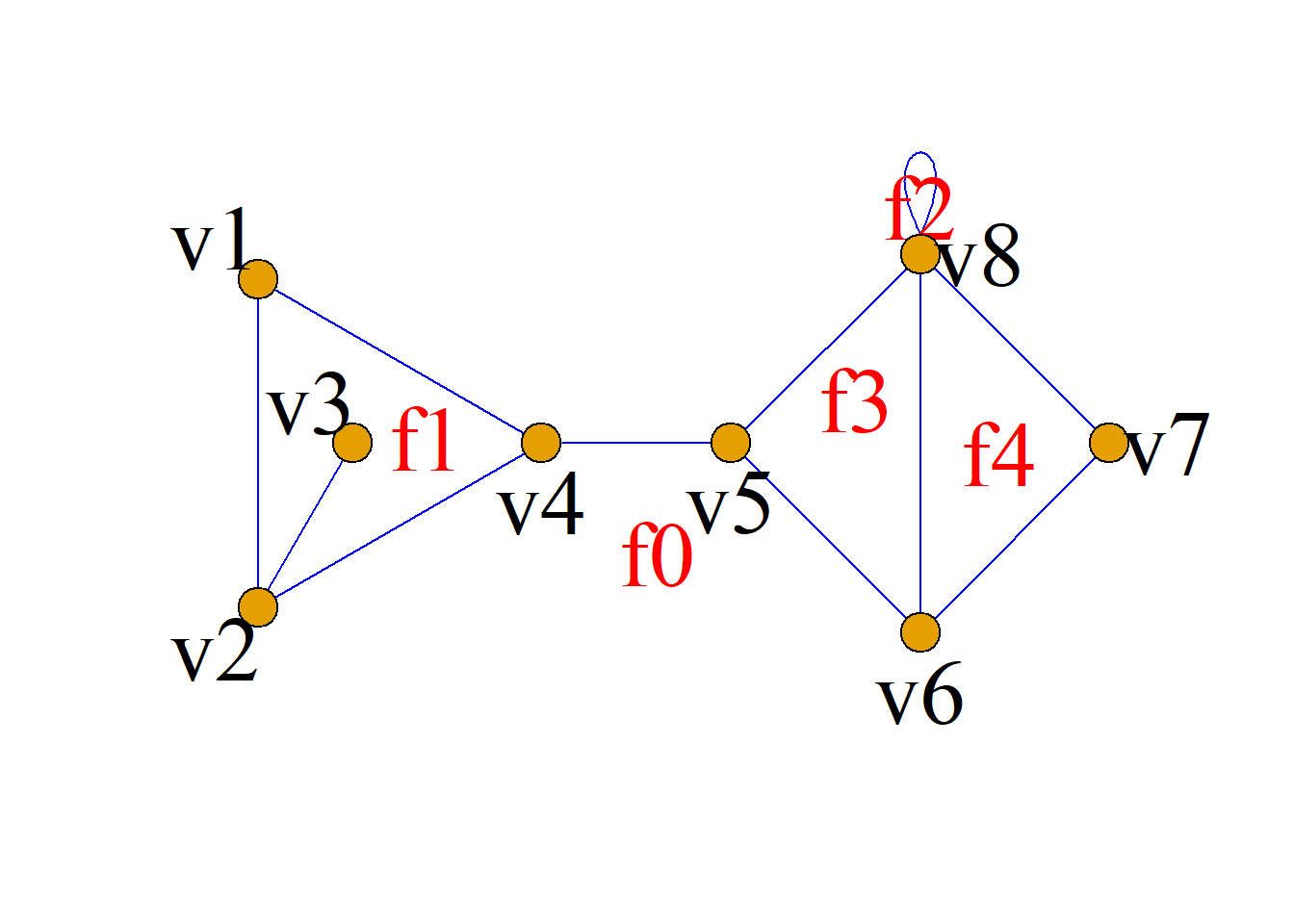
Example: As shown in the figure, it is a planar figure, which has 5 faces \(f_1, f_2, f_3, f_4\) and \(f_0\), among which \(f_0\) is an infinite face and the rest are finite faces.
The boundary of \(f_1\) is \((v_1, v_2, v_3, v_2, v_4, v_1)\), and the degree is 5;
The boundary of \(f_2\) is \((v_8, v_8)\), and the degree is 1;
The boundary of \(f_3\) is \((v_5, v_6, v_8, v_5)\), and the degree is 3;
The boundary of \(f_4\) is \((v_6, v_7, v_8, v_6)\), and the degree is 3;
The boundary of \(f_0\) is \((v_1, v_2, v_4, v_5, v_6, v_7, v_8, v_8, v_5, v_4, v_1)\), and the degree is 10.
Theorem: In a connected planar graph \(G={\langle}V, E, F{\rangle}\), the sum of the degrees of all faces is equal to twice the number of sides, that is, \(=2|E|\).
Proof: Because any edge connecting the planar graph either appears once as a common edge of the two faces in the boundary of the two faces, or appears twice in the boundary of one face.
No matter which of the two cases it is, the degree of each face is calculated twice, so the sum of the degrees of all faces is equal to twice the number of sides.
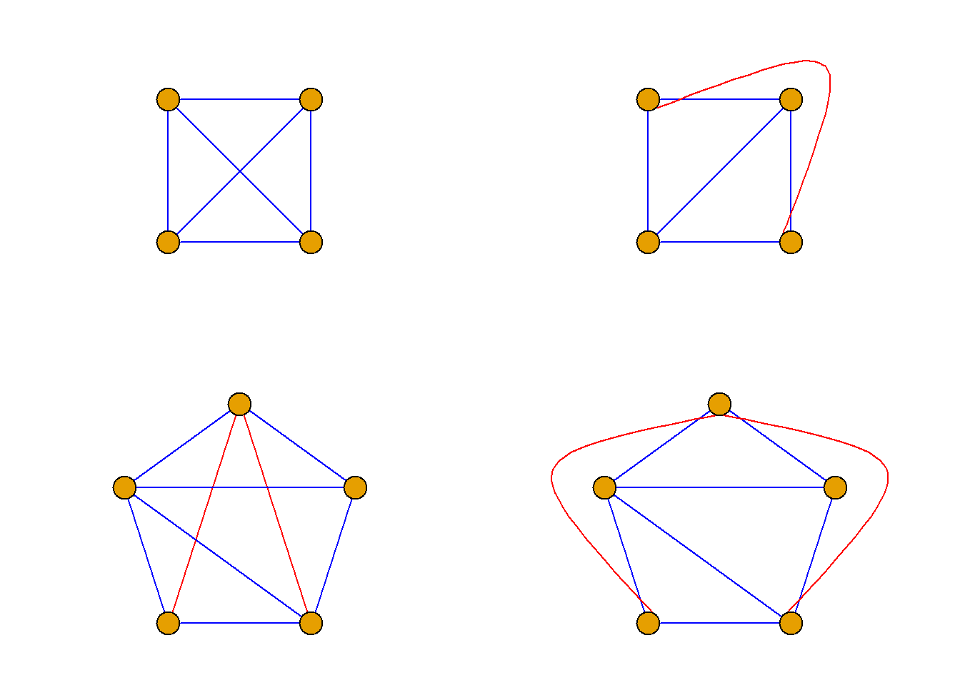
Definition: Assume that the simple graph \(G\) is a planar graph. If an edge is added between any two non-adjacent nodes in \(G\), the resulting graph will be a non-planar graph, then \(G\) is said to be a maximum planar graph.
Maximal planar graphs must be connected, and the boundaries of each surface are composed of basic circuits.
The undirected complete graphs \(k_3\) and \(k_4\) are both maximal planar graphs.
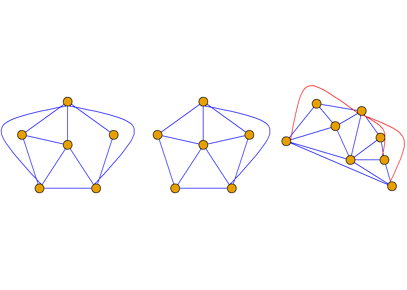
Theorem: For a simple connected plane graph \(G\) with the number of nodes greater than or equal to 3, \(G\) is a maximum plane graph if and only if the degree of each face in \(G\) is 3.
Example: In the figure, which are the maximum planar plans?
Only the graph on the right is a maximal planar graph, because only the degree of each face of this graph is 3.
Definition: Suppose \(G\) is a non-planar graph. If any edge in \(G\) is deleted, the resulting graph is a planar graph, then \(G\) is said to be a minimum non-planar graph.
Minimal non-planar graphs must be simple graphs.
\(K_5\) and \(K_{3, 3}\) are both minimal non-planar graphs.
Theorem: (Euler’s formula) Suppose \(G\) is a connected planar graph with \(n\) nodes, \(m\) edges and \(r\) faces, then \(n-m+r=2\).
Example: In the picture \[n-m+r=4-5+3=2.\]
Example: Suppose the connected plane graph \(G\) has 20 nodes, and the degree of each node is 3. How many faces does the plane representation of this plane graph divide the plane into?
Solution: Suppose \(G={\langle}V, E{\rangle}={\langle}n, m{\rangle}\), then \(n=20\), so the sum of the degrees of all nodes \({\sum}d(v)=3n=3{\times}20=60\). And since the sum of the degrees of the nodes \({\sum}d(v)=2m=60\), that is, \(m=30\).
According to Euler’s formula, the number of faces is: \[r=2-n+m=2-20+30=12\] According to Euler’s formula, some inequalities of plane graphs can be obtained.
Theorem: Suppose \(G\) is a planar graph with \(n\) nodes connected to \(m\) edges. If the degree of each surface is greater than or equal to \(l\), here \(l{\geq}3\), then: \[m{\leq}\frac{l(n-2)}{l-2}\] Proof: Suppose \(G\) has r faces, then it can be known from the problem:
\[ 2m=\sum_f{deg(f){\geq}l{\cdot}r} \]
And according to Euler’s formula \(n-m+r=2\), there is \(r=2-n+m\). Therefore, \(2m{\geq}l(2-n+m)\).
Then from \(l{\geq}3\), we get \(m{\leq}\frac{l(n-2)}{l-2}\).
Theorem: Suppose \(G\) is a simple plane graph with \(n\) nodes and \(m\) connected edges. If \(n{\geq}3\), then \(m{\leq}3n-6\).
Obviously this is a necessary condition for a floor plan, but it is not a sufficient condition.
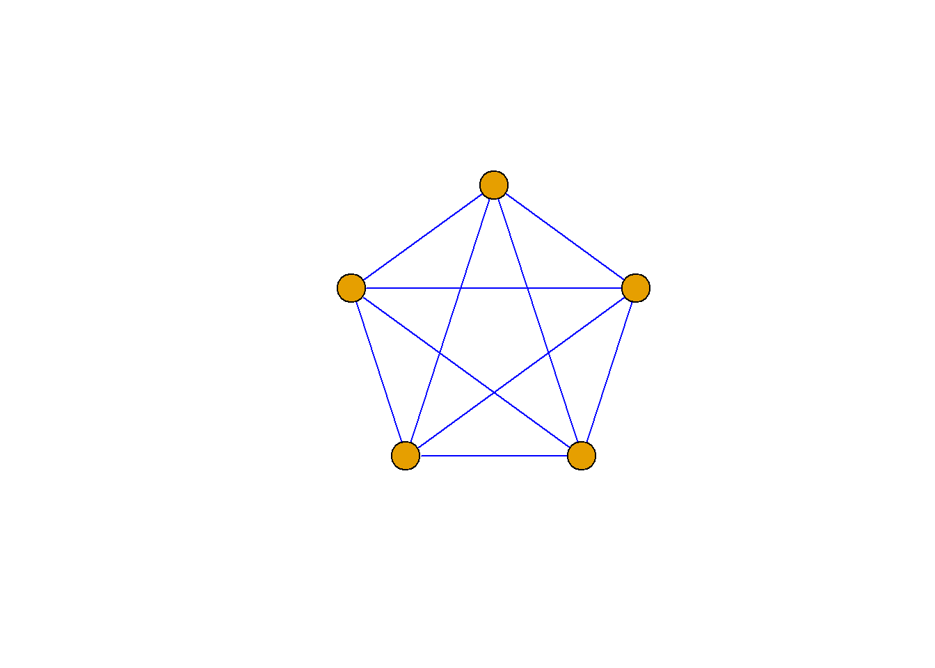
Prove: \(k_5\) is a non-planar graph.
Proof: Proof by contradiction. Suppose \(k_5\) is a planar graph. Since the number of nodes \(n=5\) and the number of edges \(m=10\) in \(k_5\), there should be \(10{\leq}3{\times}5-6=9\). Obviously this is not true, so the assumption is not true and \(k_5\) is a non-planar graph.
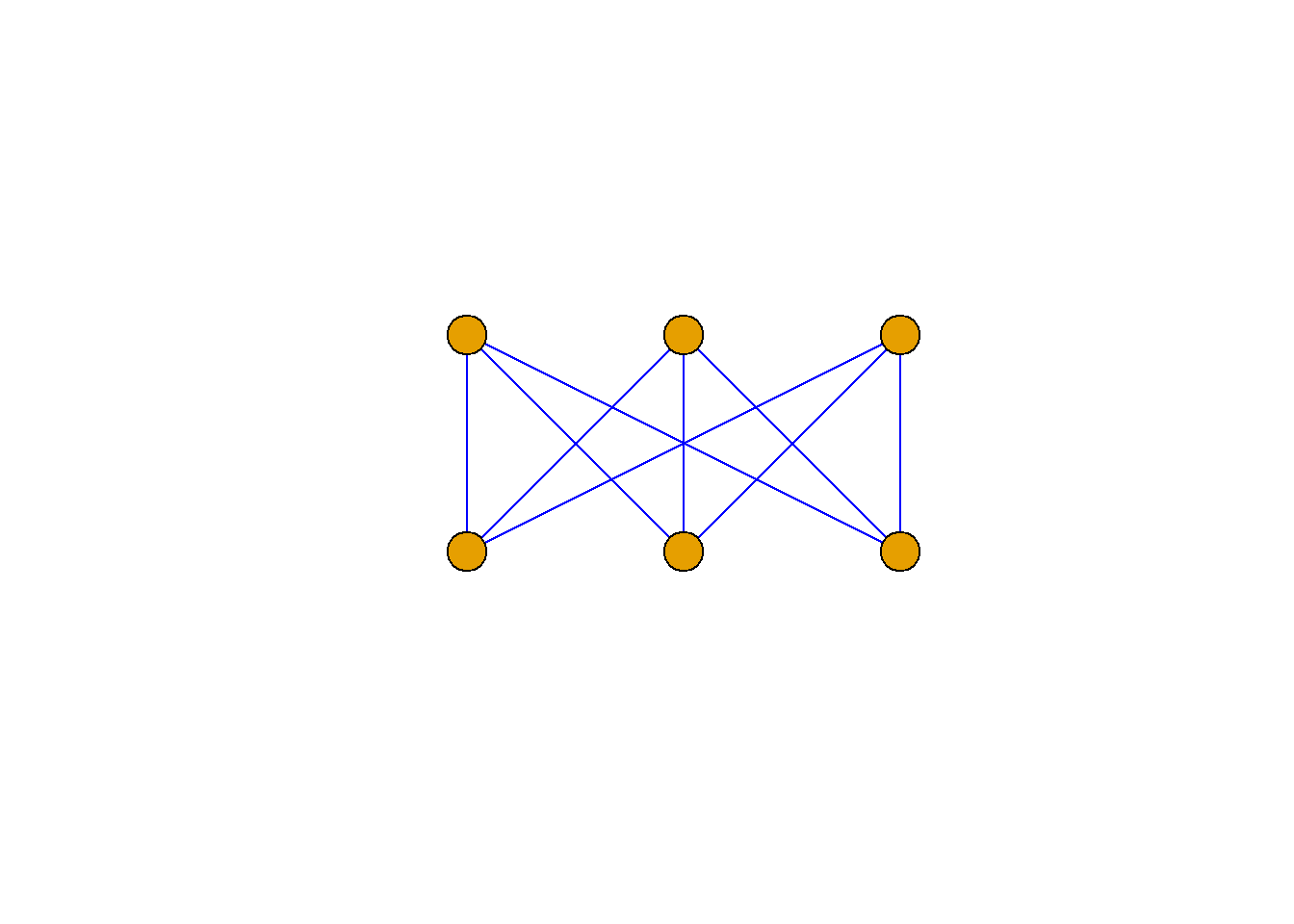
For \(k_{3, 3}\), it is impossible to determine whether it is a planar graph. Because: the number of nodes \(n=6\) of \(k_{3, 3}\), the number of edges \(m=9\), there are: \[m=9{\leq}3n-6=3{\times}6-6=12, \] That is, it satisfies \(m{\leq}3n-6\), so it cannot be determined whether \(k_{3, 3}\) is a planar graph.
Theorem: Suppose \(G\) is a simple plane graph with \(n\) nodes and \(m\) connected edges. If \(n{\geq}3\) and there is no loop of length 3 in \(G\), then: \[m{\leq}2n-4.\]
Proof: Suppose \(G\) has \(r\) faces.
Since there is no loop of length 3 in \(G\), the degree of each face of \(G\) is at least 4, so there is \(2m{\geq}4r\), that is, \(r{\leq}m/2\).
According to Euler’s formula \(n-m+r=2\), we have: \(m-n+2=r{\leq}m/2\). Therefore, \(m{\leq}2n-4\).
Obviously this is also a necessary condition, but not a sufficient condition.
Example: Prove that \(k_{3, 3}\) is a non-planar graph.
Proof: Proof by contradiction. Suppose \(k_{3, 3}\) is a plane graph.
Since the number of nodes \(n=6\) in \(k_{3, 3}\), the number of edges \(m=9\), and there is no loop of length 3, there should be \(m{\leq}2n-4\), that is, \(9{\leq}2{\times}6-4=8\). Obviously this is not true.
Therefore, the assumption does not hold, so \(k_{3, 3}\) is a non-planar graph.
Theorem: Suppose \(G\) is a simple planar graph, then the minimum degree of \(G\) is \(\delta(G){\leq}5\).
Proof: If the number of nodes \(n{\leq}6\), the conclusion is obviously true.
If the number of nodes \(n{\geq}7\), use proof by contradiction.
Assuming \(\delta(G){\geq}6\), we can know from the handshake theorem:
\[2m=\sum_{v{\in}V}d(v){\geq}6n.\]
Therefore \(m{\geq}3n\), which is contradictory to \(m{\leq}3n-6\). Therefore, the assumption does not hold, that is, the minimum degree of \(G\) is \(\delta(G){\leq}5\).
This theorem is related to the coloring theory of graphs.
Euler’s formula inference: Assume that the plane graph \(G\) has \(k(k{\geq}2)\) connected branches, then: \(n-m+r=k+1\). Among them, \(n, m, r\) are the number of nodes, edges and faces of \(G\) respectively.
Proof: Assume that the \(i\)th connected branch has \(n_i\) nodes, \(m_i\) edges and \(r_i\) faces, and use Euler’s formula for each connected branch: \[n_i-m_i+r_i=2\] Sum: \((n_1+n_2+{\cdots}n_k)-(m_1+m_2+{\cdots}m_k)+(r_1+r_2+{\cdots}r_k)=2k\).
Note that \(r=r_1+{\cdots}+r_k-(k-1)\) (there is only one external surface), we get: \(n-m+r=k+1\).
Theorem: Suppose the plane graph \(G\) has \(k(k{\geq}2)\) connected branches, and the degree of each face is at least \(l(l{\geq}3)\), then the number of edges \(m\) and the number of nodes \(n\) have the following relationship:
\[ m{\leq}\frac{l}{l-2}(n-k-1) \]
Identification of floor plan
The search for necessary and sufficient conditions for judging floor plans lasted for decades until 1930, when Kazimierz Kuratowski took the lead in solving this problem by giving a very simple feature of floor plans.
Insert or delete a node with degree 2:
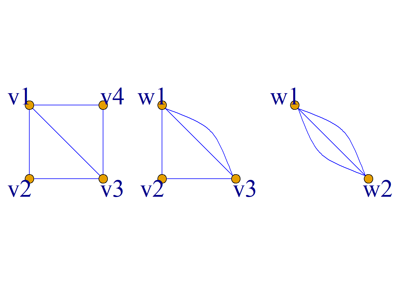
As shown in Figure \(G\), it can be seen that on the edge of a given graph \(G\), insert a new node with degree 2, so that one edge is divided into two edges;
Or delete the node with degree 2 and combine the two edges into one edge. None of these will affect the planarity of the graph.
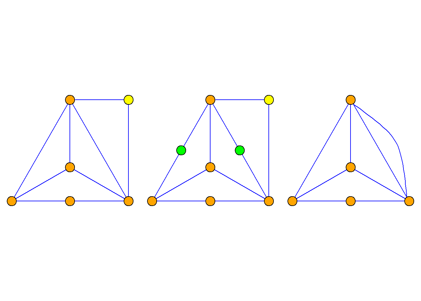
Definition: Given two undirected graphs \(G_1\) and \(G_2\), if \(G_1\) and \(G_2\) are isomorphic, or become isomorphic by repeatedly inserting or deleting nodes with degree 2 on some edges, then \(G_1\) and \(G_2\) are called homeomorphism.
The planarity of a graph remains unchanged in the sense of homeomorphism of the graph, that is, if any number of 2-degree nodes are inserted or deleted from a planar graph, the resulting graph will still be a planar graph.
Theorem (Kuratowski’s Theorem I): An undirected graph \(G\) is a planar graph if and only if \(G\) does not contain a subgraph homeomorphic to \(k_5\) or \(k_{3, 3}\).
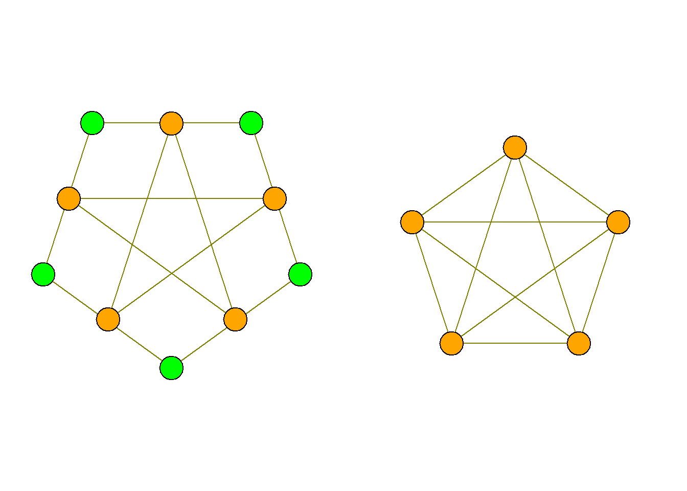
Definition: In an undirected graph \(G\),
Remove two adjacent nodes \(u, v\) and their associated edges \((u, v)\) in \(G\),
Replace it with a new node \(w\), so that \(w\) is adjacent to all nodes adjacent to \(u and v\),
Performing a series of such transformations on \(G\) results in a new graph \(G^{\prime}\), which is called the basic condensation of \(G\).
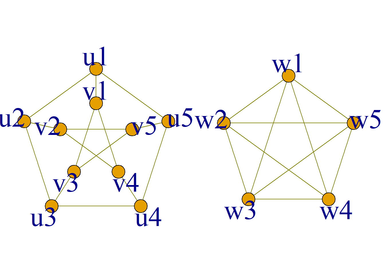
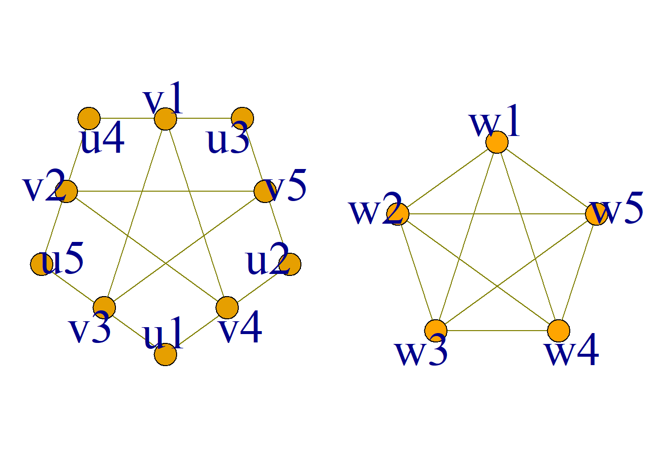
Theorem (Kuratowski’s Theorem II):
An undirected graph \(G\) is a planar graph if and only if there is no subgraph in \(G\) that can be condensed to \(k_5\) or \(k_{3, 3}\).
Dual graph
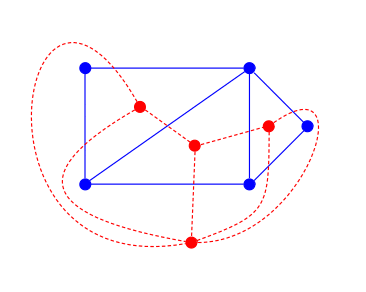
Definition: Assume \(G\) is a planar graph, the undirected graph \(G^*\) constructed by the following method is called the dual graph of \(G\).
Pick any point \(v_i^*\) in each face \(f_i\) of \(G\) as the node of \(G^*\).
If in \(G\), the boundaries of faces \(f_i\) and \(f_j\) have a common edge \(e_k\), then connect the corresponding nodes \(v_i^*\) and \(v_j^*\), so that the edge \(e_k^*\) of \(G^*\) intersects with \(e_k\), and does not intersect with other edges of \(G\).
If in \(G\), \(e_k\) only appears on the boundary of one face \(f_i\), the ring \(e_k^*\) of \(G^*\) from the corresponding node \(v_i^*\) to \(v_i^*\) intersects with \(e_k\), and does not intersect with other edges of \(G\).
Theorem: Every connected plane graph \(G\) has its dual graph, and the dual graph \(G^*\) of a connected plane graph \(G\) is also a connected plane graph. In addition, \(G^*\) is also the dual graph of \(G\).
For isomorphic planar graphs, their dual graphs are not necessarily isomorphic.
For example, the two graphs in the figure are isomorphic, but their dual graphs are not.
Because the maximum degree of the left picture is 6, and the maximum degree of the right picture is 5.
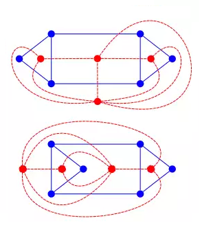
Theorem: The number of nodes \(n\), the number of edges \(m\) and the number of faces \(r\) of a connected planar graph \(G\) has the following relationship with the number of nodes \(n^*\), the number of edges \(m^*\) and the number of faces \(r^*\) of its dual graph \(G^*\): \[n=r^*, m=m^*, r=n^*\]
As shown in the figure, \[n=r^*=5\] \[m=m^*=7\] \[r=n^*=4\]
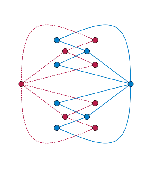
Definition: If the dual graph \(G^*\) of the plane graph \(G\) is isomorphic to \(G\), then \(G\) is said to be a self-dual graph.
The graph shown in the figure is a self-dual graph.
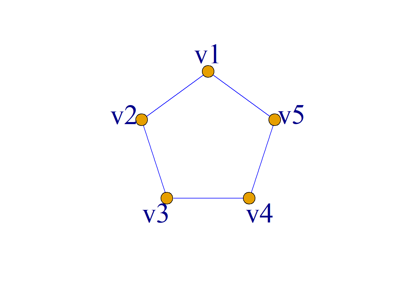
Definition: A graph composed of \(n\)(\(n{\geq}3\)) nodes \(v_1, v_2, {\cdots}, v_n\), and edges \((v_1, v_2), (v_2, v_3), {\cdots}, (v_{n-1}, v_n), (v_n, v_1)\) is called cyclic graph, denoted as \(C_n\).
Example: As shown in the figure, it is a circle chart.
The number of nodes contained in graph \(G\) is called the order of graph \(G\).
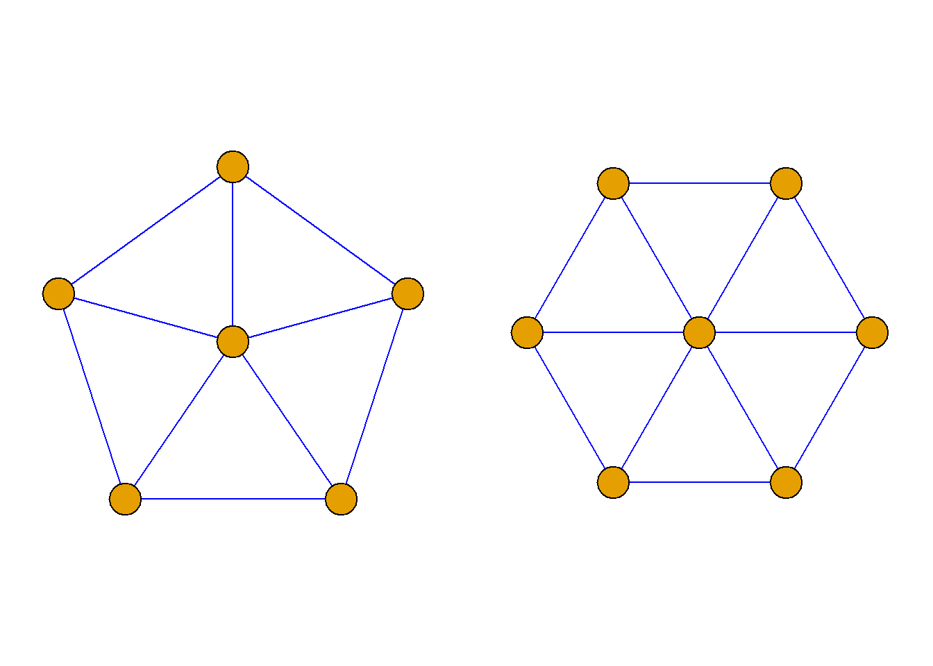
Definition: Place a point in the cycle graph \(C_{n-1}\) so that this point is adjacent to all nodes on \(C_{n-1}\). The resulting \(n\)-order simple graph is called n-order wheel graph. Denoted as \(W_n\).
A wheel graph with an odd number of \(n\) is called an odd-order wheel graph; A wheel graph in which \(n\) is an even number is called an even-order wheel graph.
Theorem: Wheel graphs are all self-dual graphs.
Floor plan coloring
More than a hundred years ago, the British Guthrie proposed the conjecture of using four colors to color maps. In 1976, American mathematicians Appel and Hecken used an electronic computer to prove that the four-color conjecture is true. This is the famous “four-color theorem”.
Map coloring problem: Use \(m\) colors to color the map so that each area on the map has a color and adjacent areas have different colors. How many colors are needed at least?
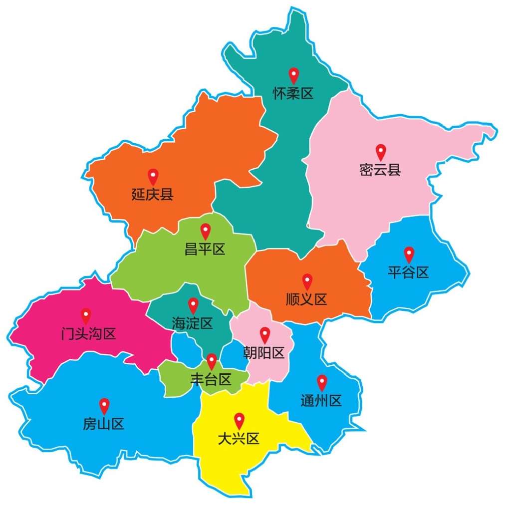
Map coloring problem: Color a map so that the number of colors is minimized.
Obviously, the map can be regarded as a planar graph, and the coloring problem of the map can be characterized by the coloring of the planar graph.
Since a planar graph has a dual graph, the problem of coloring a planar graph can be transformed into a problem of coloring the nodes of its dual graph.
Coloring classification of pictures:
Node coloring: Use \(m\) colors to color each node of the graph, requiring each node to have a color, and making two adjacent nodes have different colors.
Edge coloring: Use \(m\) colors to color each edge of the graph, requiring each edge to be colored with one color, and making two adjacent edges have different colors.
Definition: If the nodes of graph \(G\) can be colored with k colors, so that any adjacent node has a different color, then \(G\) is said to be k-colorable.
If \(G\) is \(k\)-colorable, rather than (\(k-1\))-colorable, then \(G\) is said to be of k color or the color number of \(G\) is k, recorded as \(x(G)\).
As shown in the figure,
The color number of \(G_1\) is \(x(G_1)=2\),
The color number of \(G_2\) is \(x(G_2)=4\).
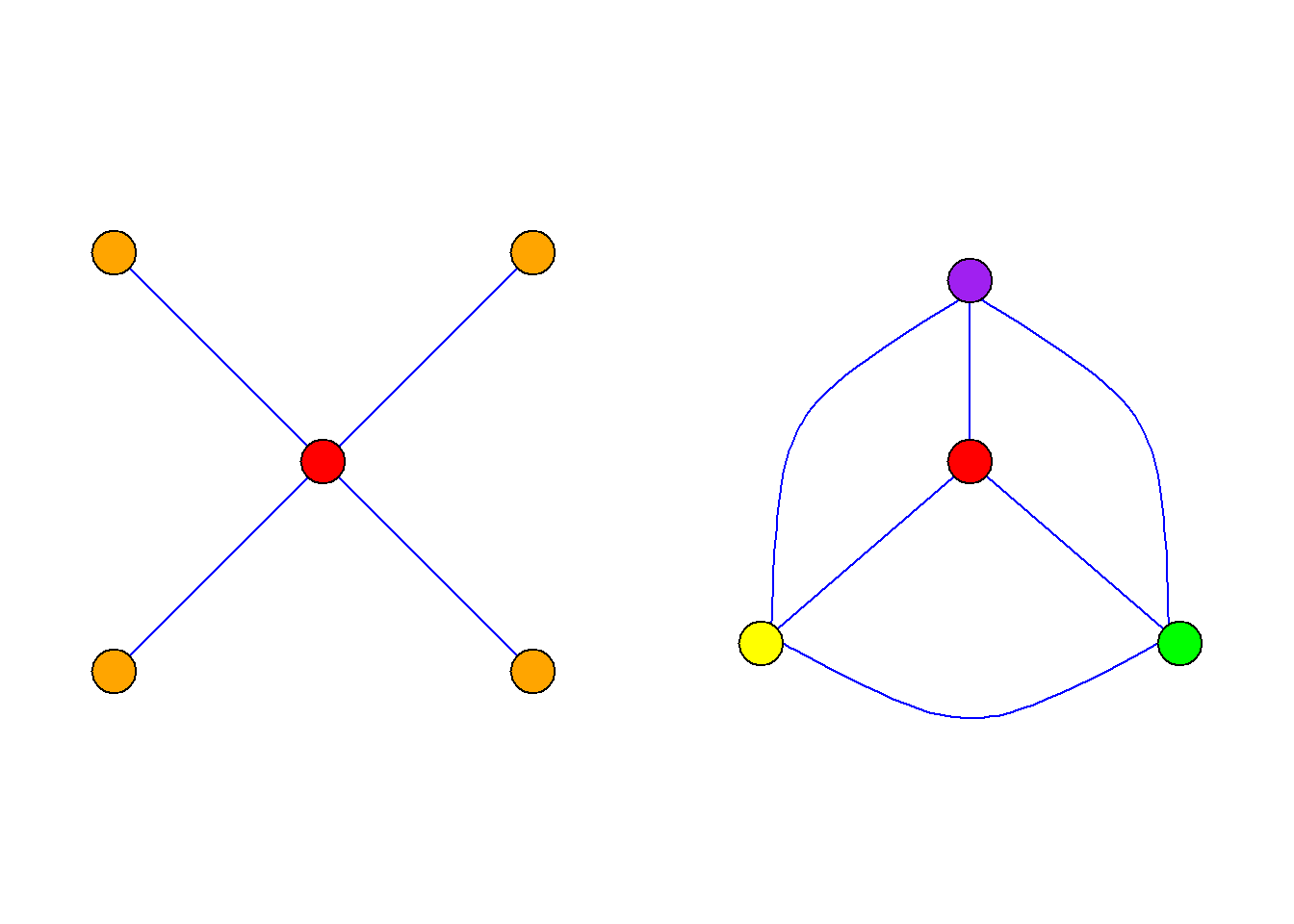
Coloring of several special figures:
\(G\) is a zero graph, and the coloring number \(x(G)=1\)
\(G\) is a complete graph with \(n\) nodes, and the coloring number \(x(G)=n\)
\(G\) is a loop with \(n\) nodes, then the coloring number \(x(G)=2\) (\(n\) is an even number); the coloring number \(x(G)=3\) (\(n\) is an odd number).
\(G\) is a non-trivial tree, and the coloring number \(x(G)=2\)
\(G\) is a bipartite graph, and the coloring number \(x(G)=2\)
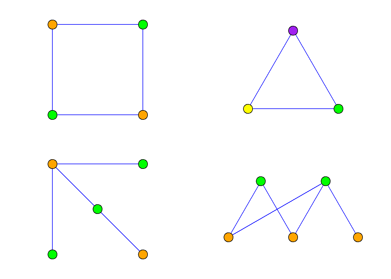
Example: Prove that the coloring number \(x(K_n)=n\) of the complete graph \(K_n\).
Proof: Because every two nodes of the complete graph are adjacent, no two nodes can be colored with the same color, so the number of colors for \(n\) nodes is not less than \(n\); and the number of colors for \(n\) nodes is at most \(n\), so \(x(K_n)=n.\)
Theorem: (Five Color Theorem) For any planar graph \(G\), there is \(x(G){\leq}5\).
Theorem: (Four Color Theorem) For any planar graph \(G\), there is \(x(G){\leq}4\). The four-color theorem only applies to planar graphs, and non-planar graphs can have arbitrarily large shading numbers.
Tree
Undirected tree and its properties
Definition: A connected undirected graph that does not contain basic circuits is called an undirected tree, or tree for short, and is often represented by \(T\). If each connected branch of an undirected graph is a tree, the graph is called a forest.
In a tree, nodes with degree 1 are called leaves, and nodes with degree greater than 1 are called branch points.
As shown in the figure, (a), (b) and (c) are all trees, (d) is a forest.
- is called trivial tree, and its node degree is 0. Only in trivial trees can there be nodes with degree 0.
In any other tree, the degree of a node is greater than or equal to 1.
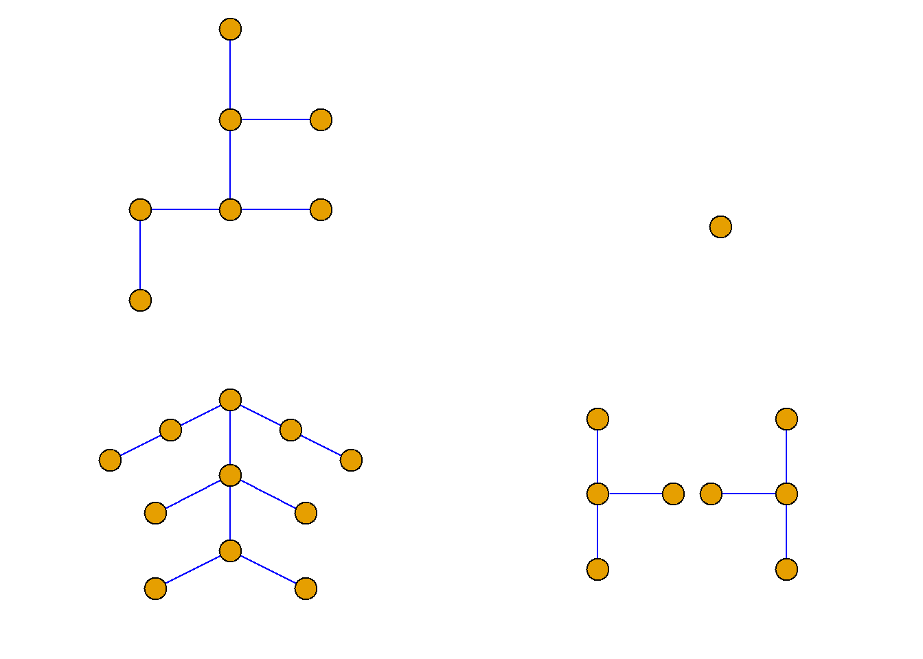
Theorem: Suppose \(G={\langle}n, m{\rangle}\) is an undirected graph, then the following propositions are equivalent and can be used as the definition of an undirected tree.
\(G\) is connected and does not contain basic circuits.
\(G\) has no basic circuit and \(m=n-1\).
\(G\) is connected and \(m=n-1\).
\(G\) has no basic cycle, but adding an edge between any two non-adjacent nodes will produce a basic cycle.
\(G\) is connected, but if any edge in \(G\) is deleted, the resulting graph will not be connected.
There is exactly one basic path between any two different nodes of \(G\).
Spanning tree
Definition: If the generating subgraph \(T\) of the undirected graph \(G\) is a tree, then \(T\) is said to be the spanning tree of \(G\).
The edges in \(T\) are called branches, and the edges of the graph \(G\) that are not in \(T\) are called chords.
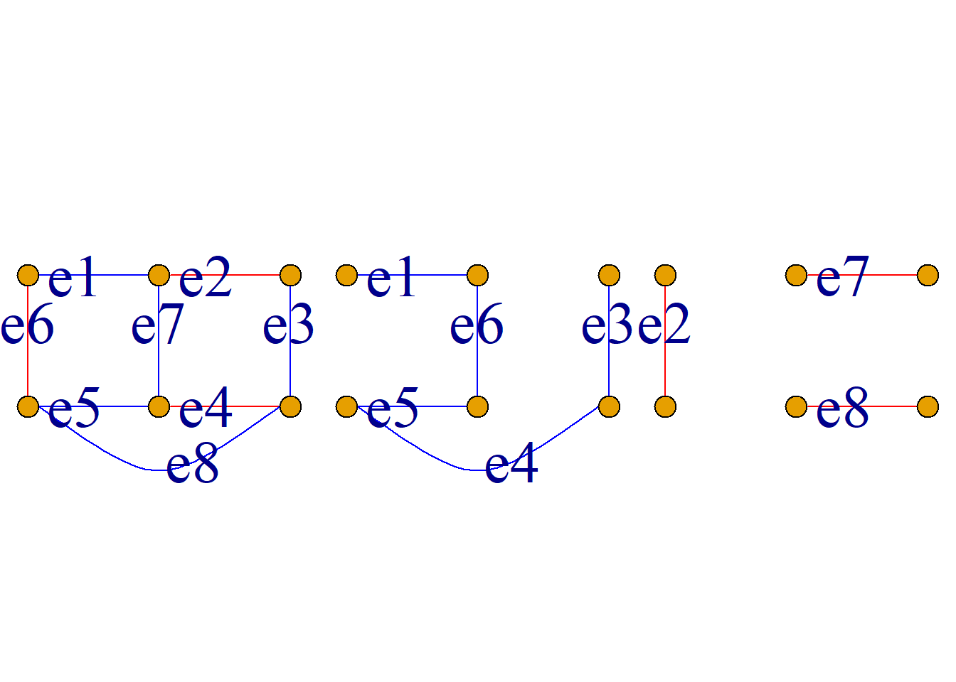
The spanning tree is not necessarily unique. As shown in Figure \(T_1\), it is another spanning tree of \(G\).
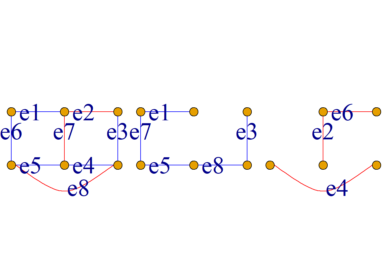
Theorem: Any connected undirected graph has at least one spanning tree.
Proof: Suppose \(G\) is a connected undirected graph. If there is no basic cycle in \(G\), then \(G\) itself is a spanning tree.
If there is a basic loop in \(G\), then delete one edge in the loop to obtain the graph \(G_1\). If there is no basic loop in \(G_1\), then \(G_1\) is a spanning tree.
If there is a basic loop in \(G_1\), then delete an edge in the loop to get the graph \(G_2\), \({\cdots}\)
This continues until there are no more basic loops in the graph. At this time, the obtained connected graph without basic loops and having the same node set as the graph \(G\) is the spanning tree of \(G\).
A connected undirected graph \(G\), if it itself is a tree, then its spanning tree is unique, which is \(G\) itself.
A connected undirected graph \(G\) itself is not a tree, and its spanning tree is not unique, but all connected undirected graphs have spanning trees.
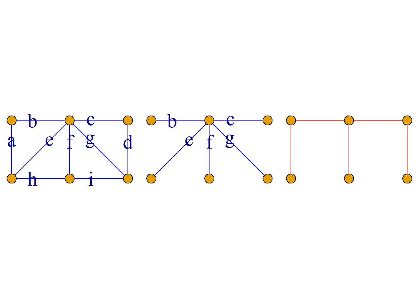
Example: As shown in the figure, in (a), the spanning tree (b) is obtained by successively deleting the edges \(a, d, h\), and \(i\), and the spanning tree (c) is obtained by successively deleting the edges \(e, g, h\), and \(i\).
Theorem: Suppose \(G={\langle}n, m{\rangle}\) is an undirected connected graph, then \(m{\geq}n-1\).
Theorem: Suppose \(G={\langle}n, m{\rangle}\) is an undirected connected graph, \(T\) is the spanning tree of \(G\), \(T^{\prime}\) is the co-tree of \(T\), then the number of edges in \(T^{\prime}\) is \(m-n+1\).
Minimum spanning tree
Definition: Let \(G={\langle}V, E, W{\rangle}\) be a connected weighted graph, and \(W\) be the function from \(E\) to the set of non-negative real numbers.
Assume \(T\) is the spanning tree of \(G\), then the sum of the edge weights in \(T\) is called the weight of the spanning tree \(T\), denoted as \(W(T)\). The spanning tree with the smallest weight is called the Minimum Spanning Tree (Minimum Spanning Tree).
Example: (a) is a weighted graph, (b) is the minimum spanning tree of (a)
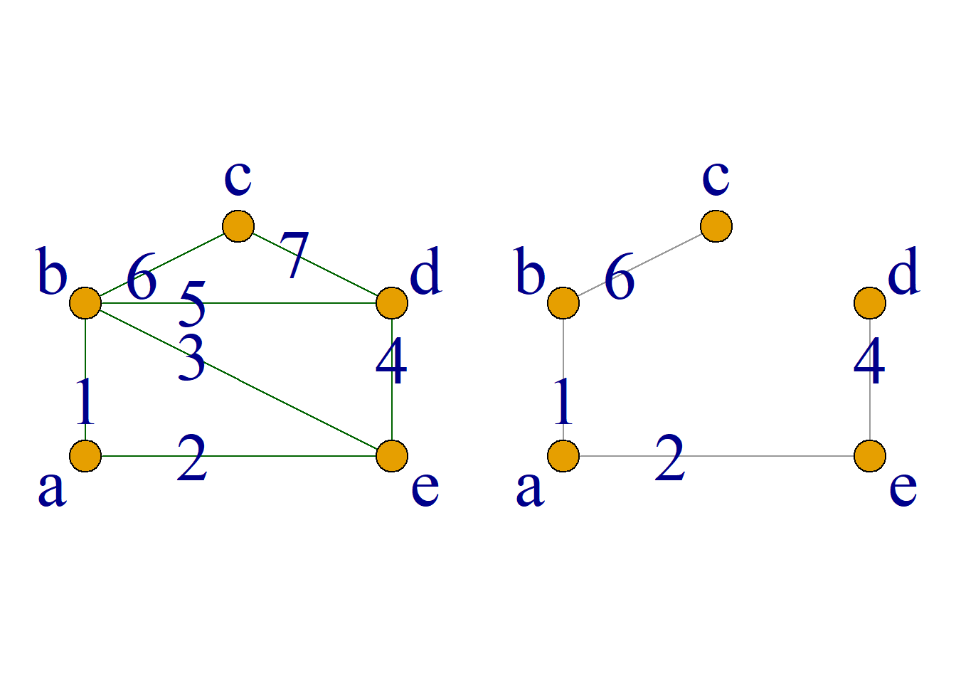
Example: Let the nodes in \(G\) represent cities, the edges represent roads between cities, and the edge weights represent the length of roads.
If communication lines are to be used to connect these cities, it is required to use the shortest line when setting up lines along the roads.
It is to require a spanning tree such that the sum of edge weights among all spanning trees in graph \(G\) is the smallest.
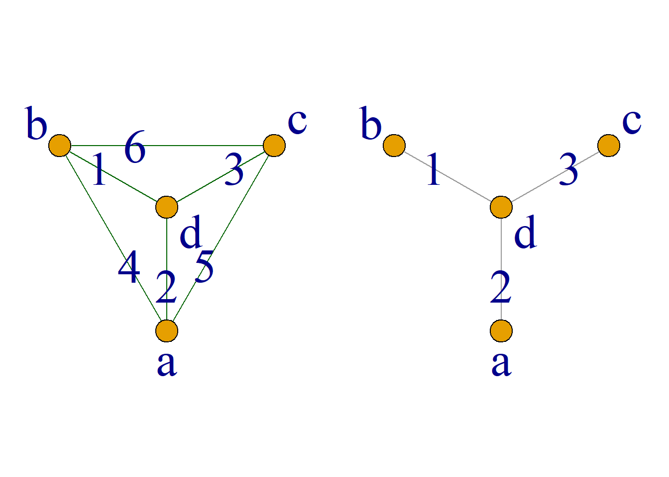
The minimum spanning tree is not necessarily unique.
As shown in the figure (a) is a weighted graph, (b) is the minimum spanning tree of (c), both of which are (a).
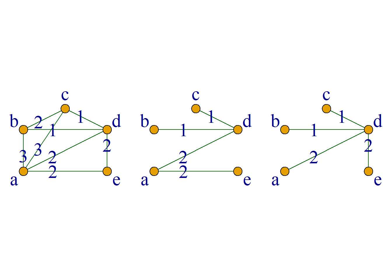
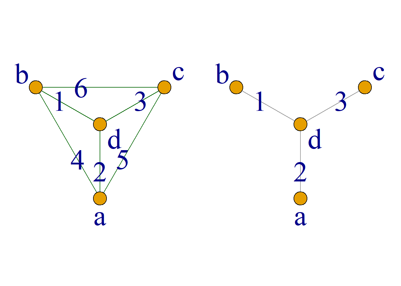
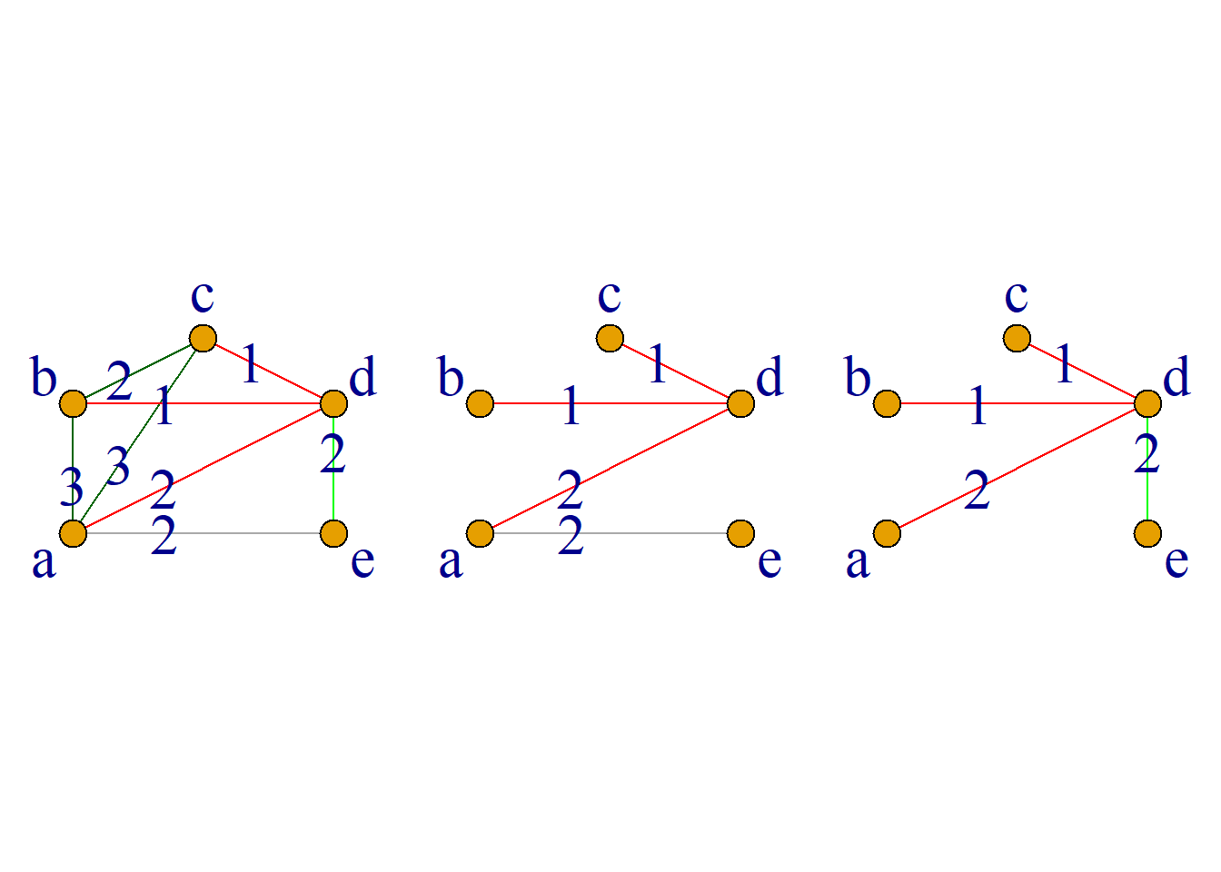
“Loop avoidance method” (Kruskal algorithm) finds the minimum spanning tree:
Assume the connected weighted graph \(G={\langle}n, m{\rangle}\), construct the graph \(T\):
The nodes of \(T\) are the same as \(G\).
Select edge \(e_1\) with the smallest possible weight in \(G\) and add it to \(T\).
Assume that edges \(e_1, e_2, {\cdots}, e_k\) have been added to \(T\). Select the edge \(e_{k+1}\) that is different from \(e_1, e_2, {\cdots}, e_k\) in \(G\), so that \(e_1, e_2, {\cdots}, e_k, e_{k+1}\) does not form a basic loop and makes the weight of \(e_{k+1}\) as small as possible, and adds \(e_{k+1}\) to \(T\).
This continues until \(n-1\) edges \(e_1, e_2, {\cdots}, e_{n-1}\) are added to \(T\).
Theorem: Suppose \(G={\langle}V, E, W{\rangle}\) is a connected weighted graph, and \(T\) obtained by Kruskal’s algorithm is the minimum spanning tree of \(G\).
Root tree and its applications
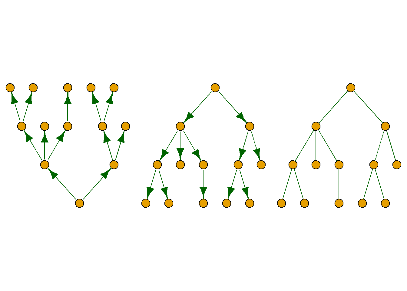
Definition: A directed graph, if the undirected graph obtained after omitting the direction of the edges is a tree, then this directed graph is called directed tree, recorded as \(T\).
Example: Graph (a) and graph (b) are both directed trees.
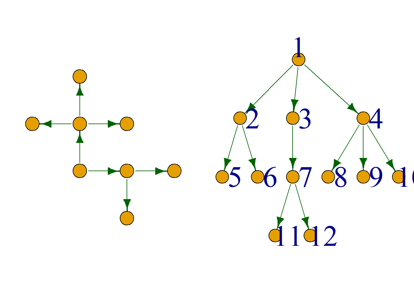
Definition: A directed tree in which only one node has an in-degree of 0 and the other nodes have an in-degree of 1 is called a root tree.
In the root tree, the node with in-degree 0 is called tree root;
A node with an in-degree of 1 and an out-degree of 0 is called a leaf;
A node whose in-degree is 1 and out-degree is not 0 is called an interior point;
Internal points and tree roots are collectively called branch points.
For example, in the root tree as shown in the figure:
\(v_1\) is the root of the tree, \(v_2, v_3, v_4, v_7\) are interior points,
\(v_5, v_6, v_8, v_9, v_10, v_{11}, v_{12}\) are leaves.
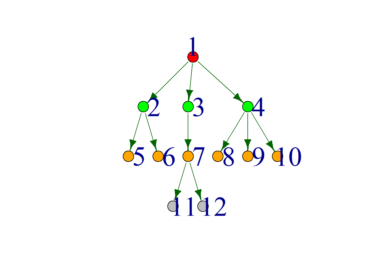
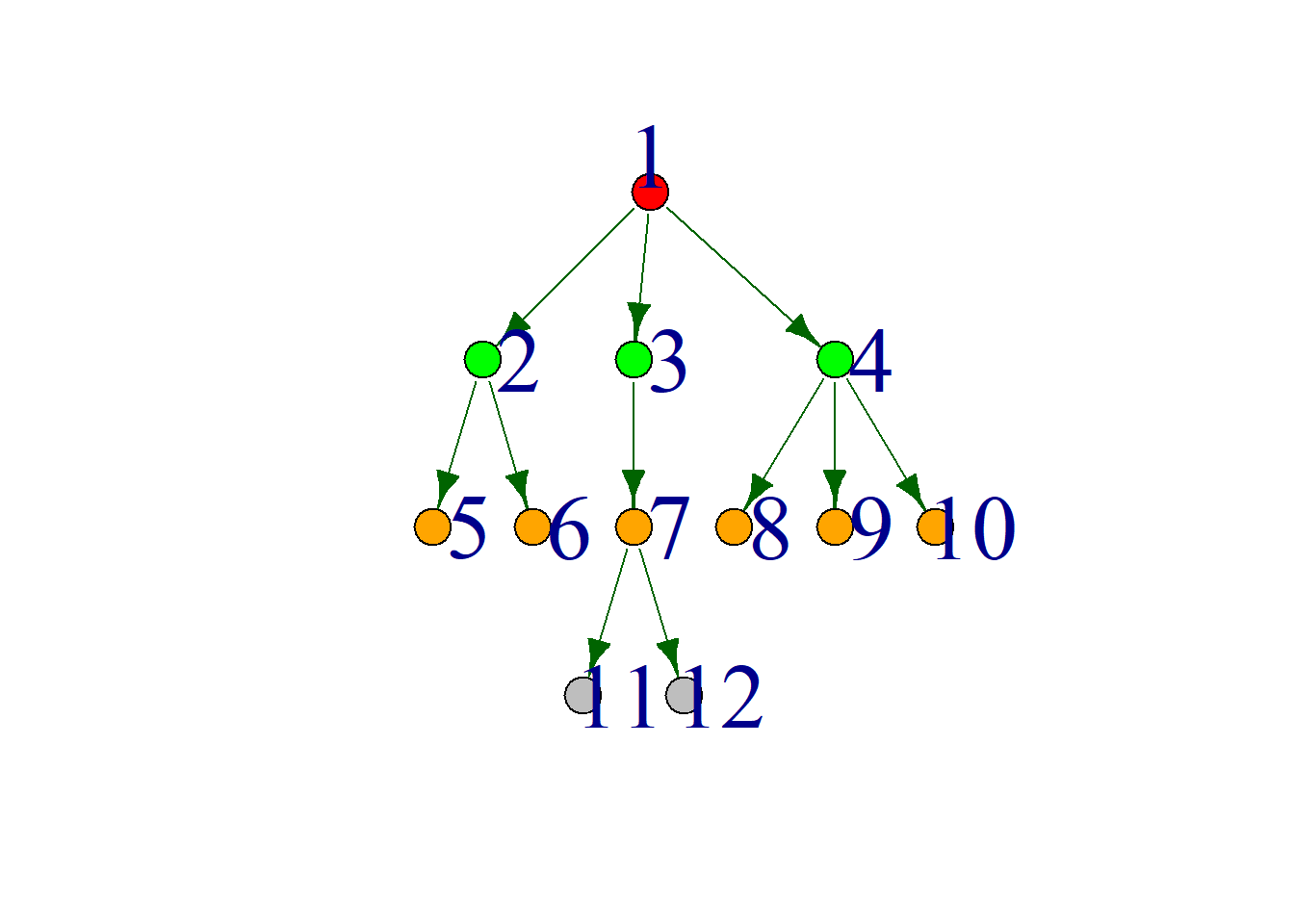
Definition: In the root tree, the path length from the root of the tree to a certain node is called the level (or layer) of the node.
Among the nodes, the maximum value of the layer is called the tree height.
For example, in the root tree as shown in the figure, the level of \(v_1\) is 0,
The level of \(v_2, v_3, v_4\) is 1,
The level of \(v_5, v_6, v_7, v_8, v_9, v_10\) is 2,
The levels of \(v_{11}, v_{12}\) are 3, and the height of the entire tree is 3.
Definition: In the root tree \(T\), if there is an edge from node \(u\) to node \(v\), then \(v\) is called the son (child node) of \(u\), and \(u\) is the father (parent node) of \(v\).
If there is a path from node \(u\) to node \(w\), then \(u\) is said to be the ancestor of \(w\), and \(w\) is the descendant of \(u\).
Nodes with the same father are called brothers.
The subgraph derived from any node \(u\) and its descendants is called a subtree with \(u\) as the root.
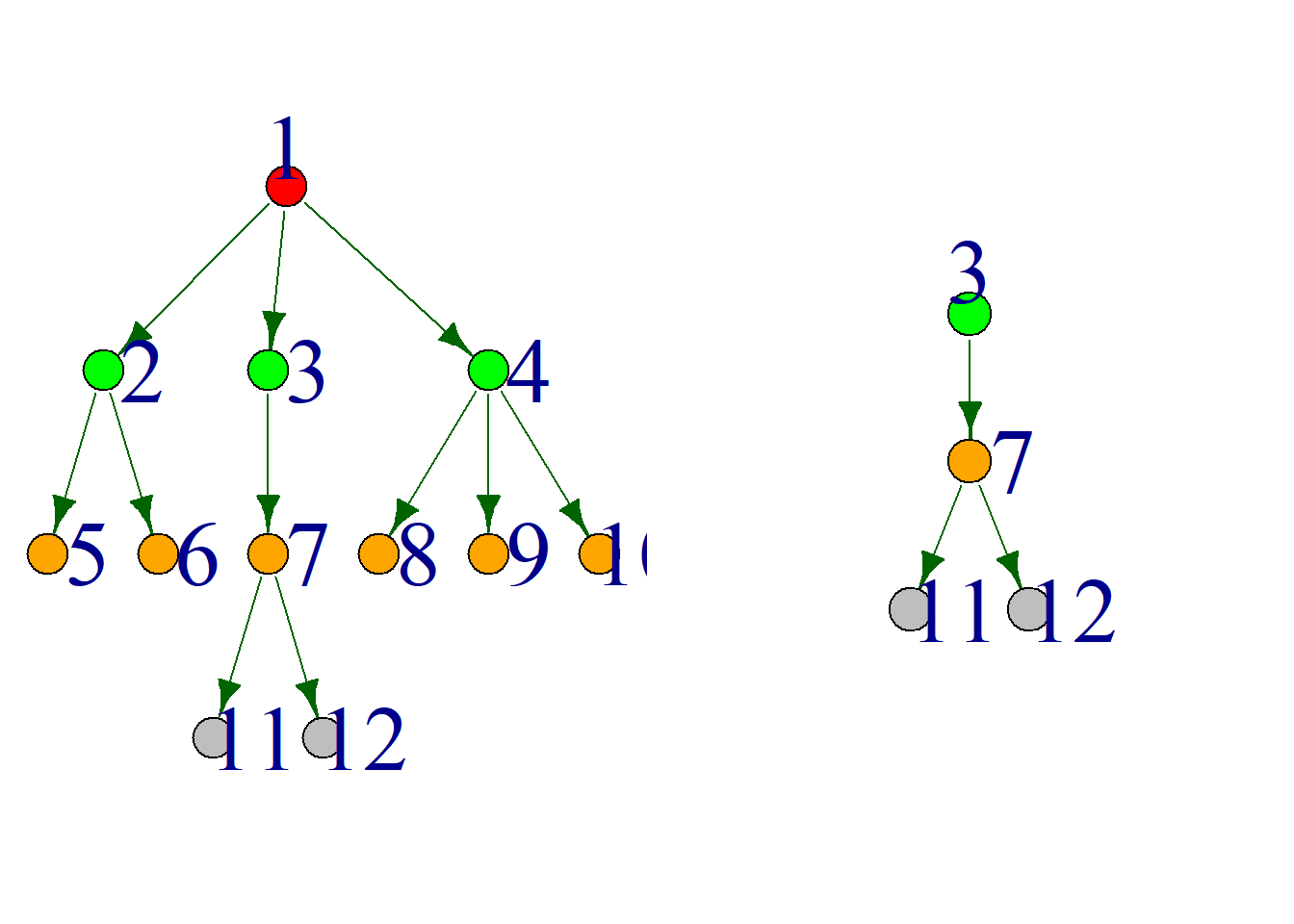
Example: As shown in the figure, \(v_8\) is the son of \(v_4\),
\(v_4\) is the father of \(v_8\),
\(v_3\) is the ancestor of \(v_{12}\),
\(v_{12}\) is the descendant of \(v_3\),
\(v_5\) and \(v_6\) are brothers.
- is the subtree of (a) with \(v_3\) as the root.
The illustration of the root tree can be arbitrary, and the roots can be drawn at any position on the root tree.
But it is generally customary to draw the roots of the tree at the upper end and the leaves at the lower end, so that the direction of the arrows pointing to the side points downward.
Therefore, all arrows can be omitted, and this method will be used later.
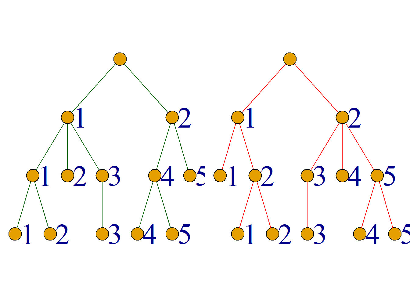
Definition: If the order of nodes on each level is specified in the root tree, such a root tree is called an ordered tree.
Generally, when drawing an ordered tree, the order of nodes on the same level is from left to right. The order of edges can also be used instead of the order of nodes.
Example: The following two trees are isomorphic as root trees, but as ordered trees, they are different.
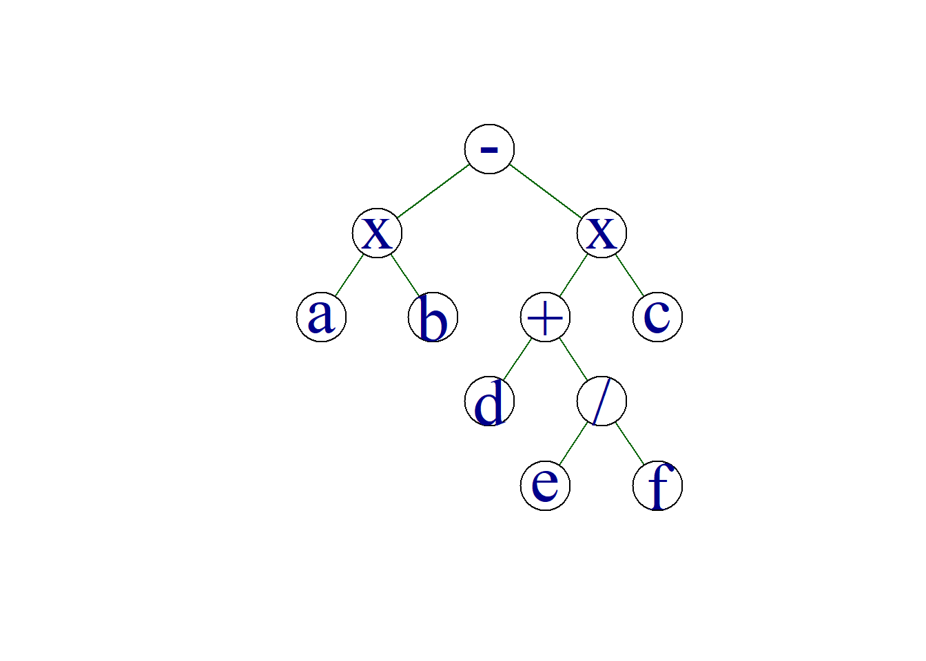
Example: As shown in the figure, the expression in the compilation principle is:
\[a{\times}b-(d+e/f){\times}c\]
The root tree is an ordered tree.
Definition: Let \(T\) be a root tree:
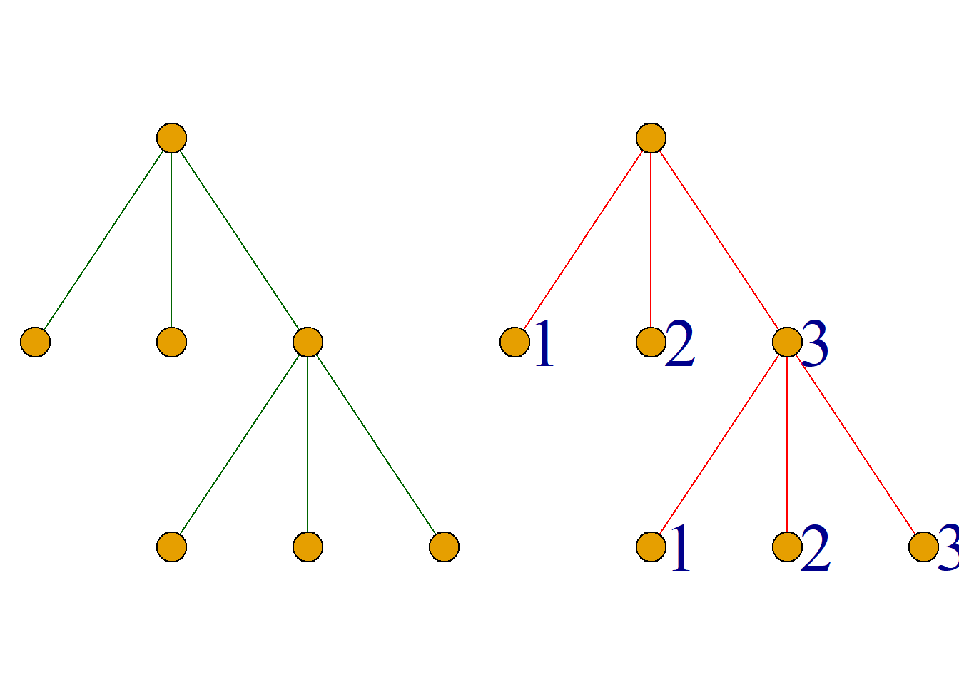
If each branch point of \(T\) has at most \(m\) sons, then \(T\) is called m-ary tree (m-ary tree); if each branch point of \(T\) has exactly \(m\) sons, then \(T\) is called regular m-ary tree.
If \(m\) fork tree \(T\) is an ordered tree, then \(T\) is called m-ary ordered tree; if regular \(m\) fork tree \(T\) is an ordered tree, then \(T\) is called regular m-ary ordered tree.
If \(T\) is a regular \(m\) tree, and all leaves have the same number of layers, then \(T\) is called a full m-tree.
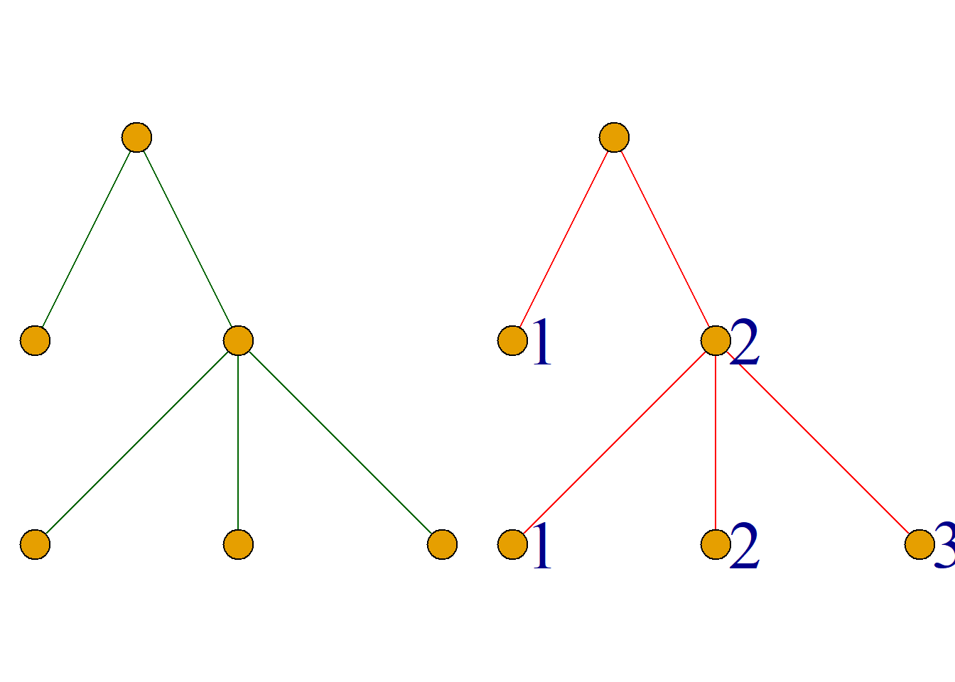
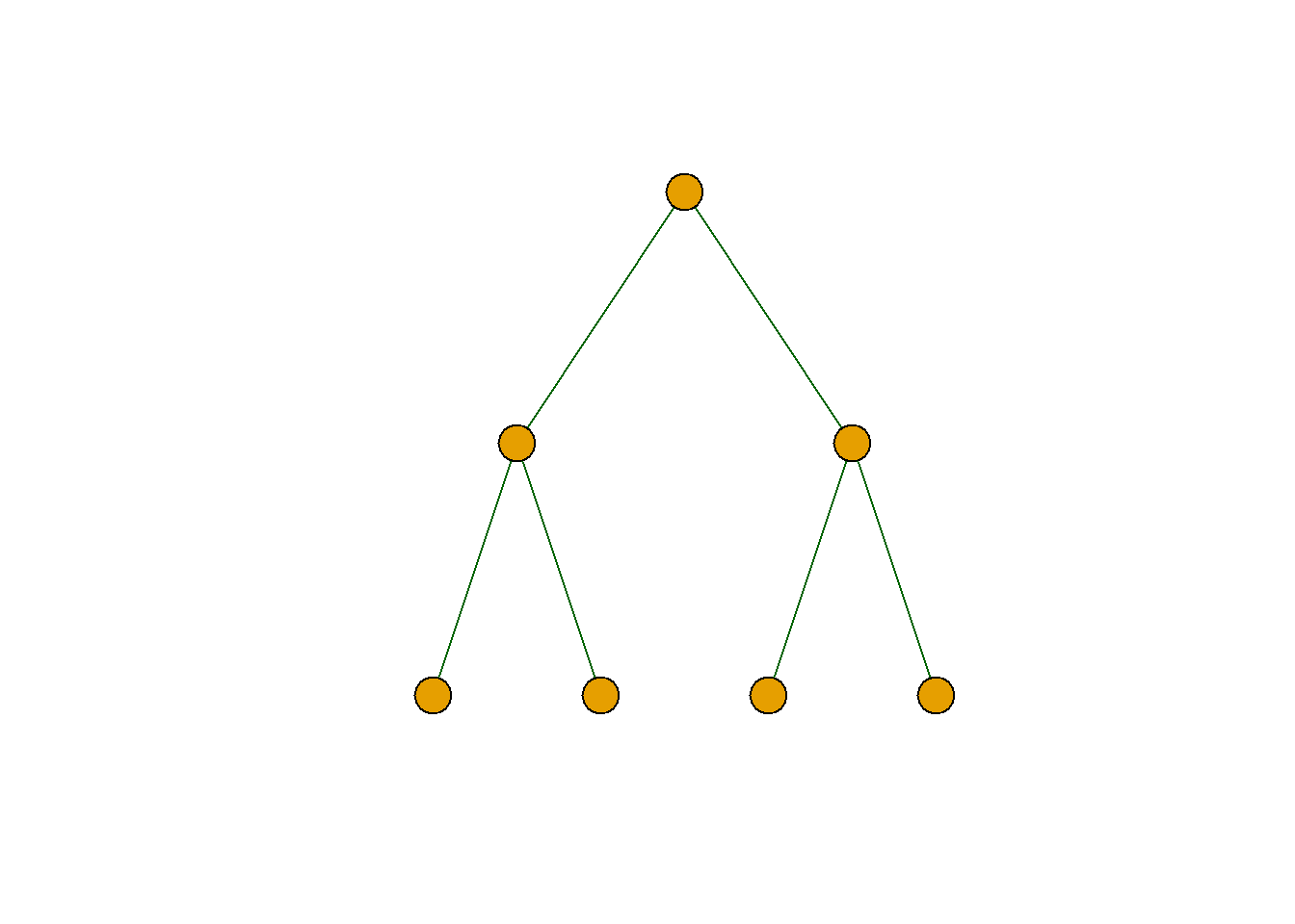
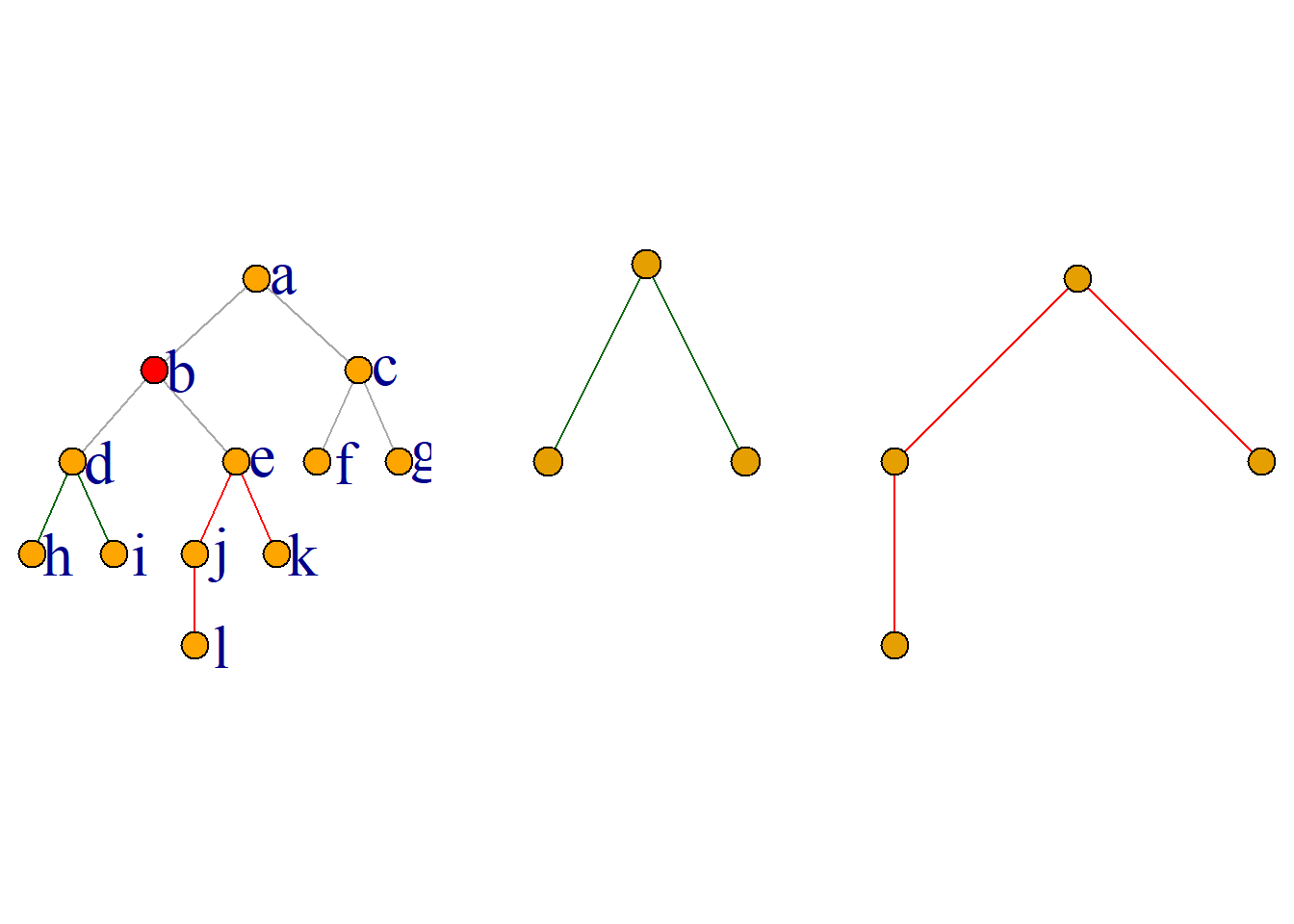
Definition: In a regular binary ordered tree, for the two sons of each branch point, the son on the left is called left son; the son on the right is called right son.
The subtree whose root is at the left child of a branch point is called the left subtree of the branch point; the subtree whose root is at the right child of a branch point is called the right subtree of the branch point.
This statement is also used for general binary ordered trees, but it should be noted that:
If a branch point of a binary ordered tree has only one son, it can be either the left son or the right son, depending on the situation.
Binary ordered trees have very important applications. Any \(m\)-ary ordered tree can be represented by the corresponding binary ordered tree. That is, any \(m\)-ary ordered tree can be transformed into a binary ordered tree by making appropriate transformations.
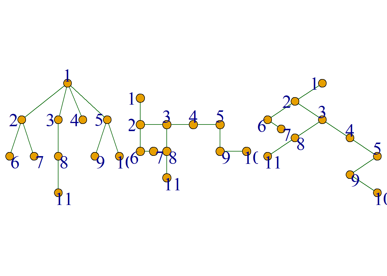
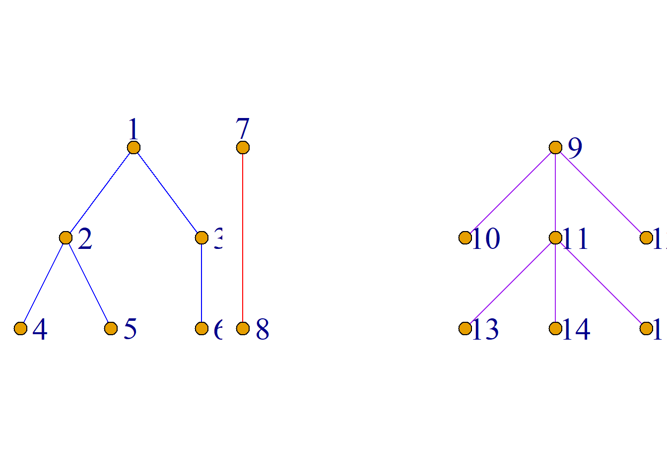
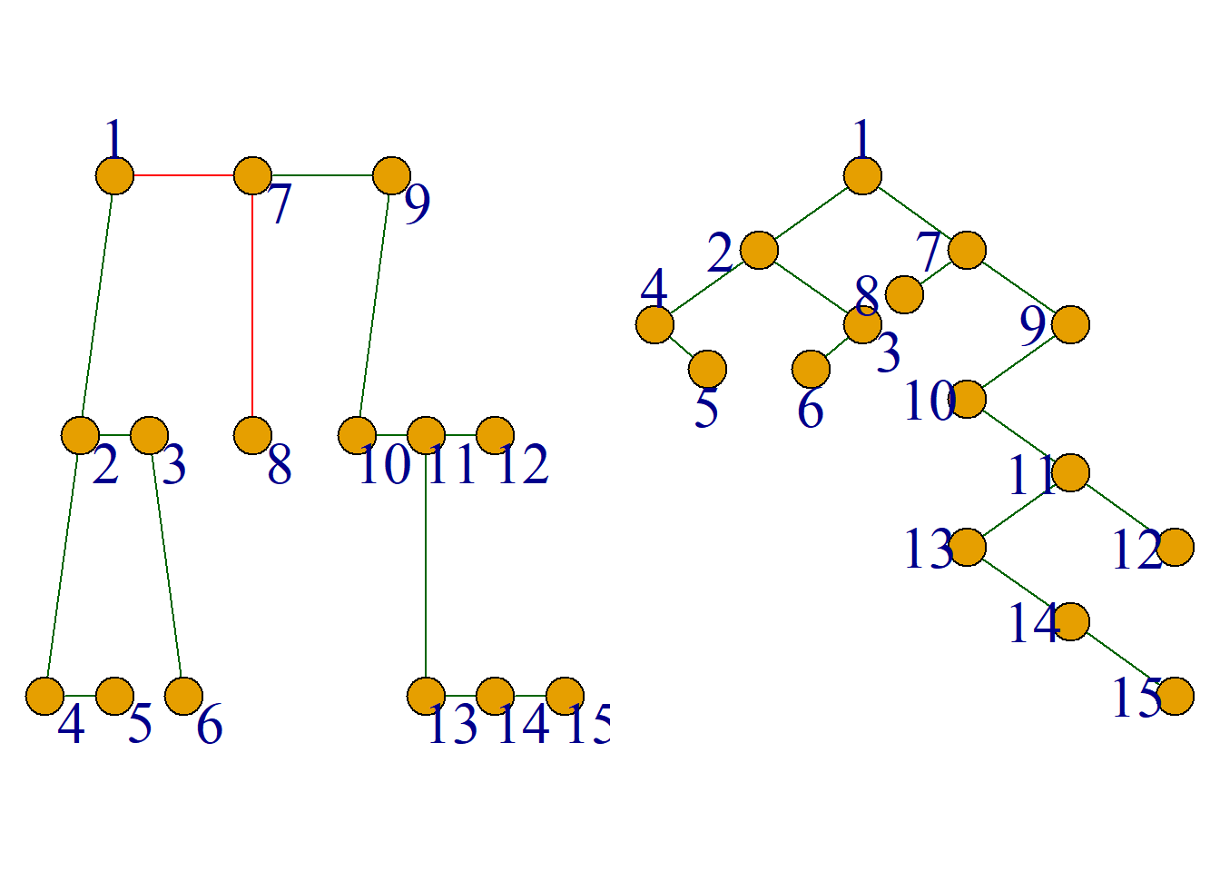
The method of converting an \(m\) element ordered tree** into a binary ordered tree** is: For an \(m\) element ordered tree, the first son of each branch point serves as the left son of the branch point, and the right sibling of the branch point (if it exists) serves as the right son of the branch point.
As shown in the figure, (a) is a 4-element ordered tree, (b) is a converted binary ordered tree, and (c) is a binary ordered tree redrawn according to the conventional graphical representation of the root tree.
Using a similar method, a binary ordered tree can be used to represent a forest composed of \(m\) ordered trees (called an ordered forest).
It can be seen from the conversion of an \(m\) element ordered tree into a binary ordered tree that the right subtree of the root of any binary ordered tree corresponding to an \(m\) element ordered tree is empty.
In this way, the ordered forest can be converted into a binary ordered tree as follows:
Represent each \(m\)-element ordered tree in the ordered forest as a binary ordered tree, and connect their tree roots in a parent-child manner, with the left being the parent and the right being the child.
An important application of binary trees: optimal binary trees.
Definition: Suppose \(T\) is a binary tree with a total of \(t\) leaves. If \(w_1, w_2, {\cdots}, w_t\) are assigned weights to these \(t\) leaves respectively, then \(T\) is called a weighted binary tree.
Definition: Suppose \(T\) is a weighted binary tree, and the weights are \(w_1, w_2, {\cdots}, w_t\), which is called \[w(t)=\sum_{i=1}^tw_il(w_i)\] is the weight of the weighted binary tree \(T\), where \(l(w_i)\) is the layer of the leaves of the weighted \(w_i\).
Among all weighted binary trees with \(t\) leaf nodes, weighted \(w_1, w_2, {\cdots}, w_t\) respectively, the one with the smallest weight is called the optimal binary tree or Huffman (Huffman)** tree**.
Theorem: Suppose \(T\) is the optimal binary tree with weights \(w_1, w_2, {\cdots}, w_t\), and \(w_1{\leq}w_2{\leq}{\cdots}{\leq}w_t\), then the leaves with weights \(w_1\) and \(w_2\) must be brothers, and they have the largest level among all nodes.
Theorem: Let \(T\) be the optimal binary tree with weights \[w_1+w_2, w_3, {\cdots}, w_t\], and \(w_1{\leq}w_2{\leq}{\cdots}{\leq}w_t\). If the leaf with weighting \(w_1+w_2\) produces two sons, weighting \(w_1\) and \(w_2\) respectively, then the obtained tree \(T^{\prime}\) is the optimal binary tree with weighting \(w_1, w_2, {\cdots}, w_t\).
According to the above two theorems, it can be seen that the optimal binary tree with \(t\) weights can be boiled down to finding the optimal binary tree with \(t-1\) weights, which can then be boiled down to finding the optimal binary tree with \(t-2\) weights, \({\cdots}\), and finally it can be boiled down to finding the optimal binary tree with 2 weights (this is the only one).
Given weights \(w_1, w_2, {\cdots}, w_t\), \(w_1{\leq}w_2{\leq}{\cdots}{\leq}w_t\), the optimal binary tree algorithm for constructing a weighted \(w_1, w_2, {\cdots}, w_t\) is as follows:
Let \(S=\{w_1, w_2, {\cdots}, w_t\}\).
Select the two weights \(w_i\) and \(w_j\) with the smallest values in \(S\), draw nodes \(v_i\) and \(v_j\), and weight \(w_i\) and \(w_j\) respectively. Draw the parent node \(v\) of \(v_i\) and \(v_j\), weight it as \(w_i+w_j\), and connect \(v_i\) and \(v\) and \(v_j\) and \(v\).
Let \(S{\leftarrow}(S-\{w_i, w_j\}){\cup}\{w_i+w_j\}\)
If \(S\) has only one element, stop and the constructed graph is the optimal binary tree. Otherwise, go to (2).
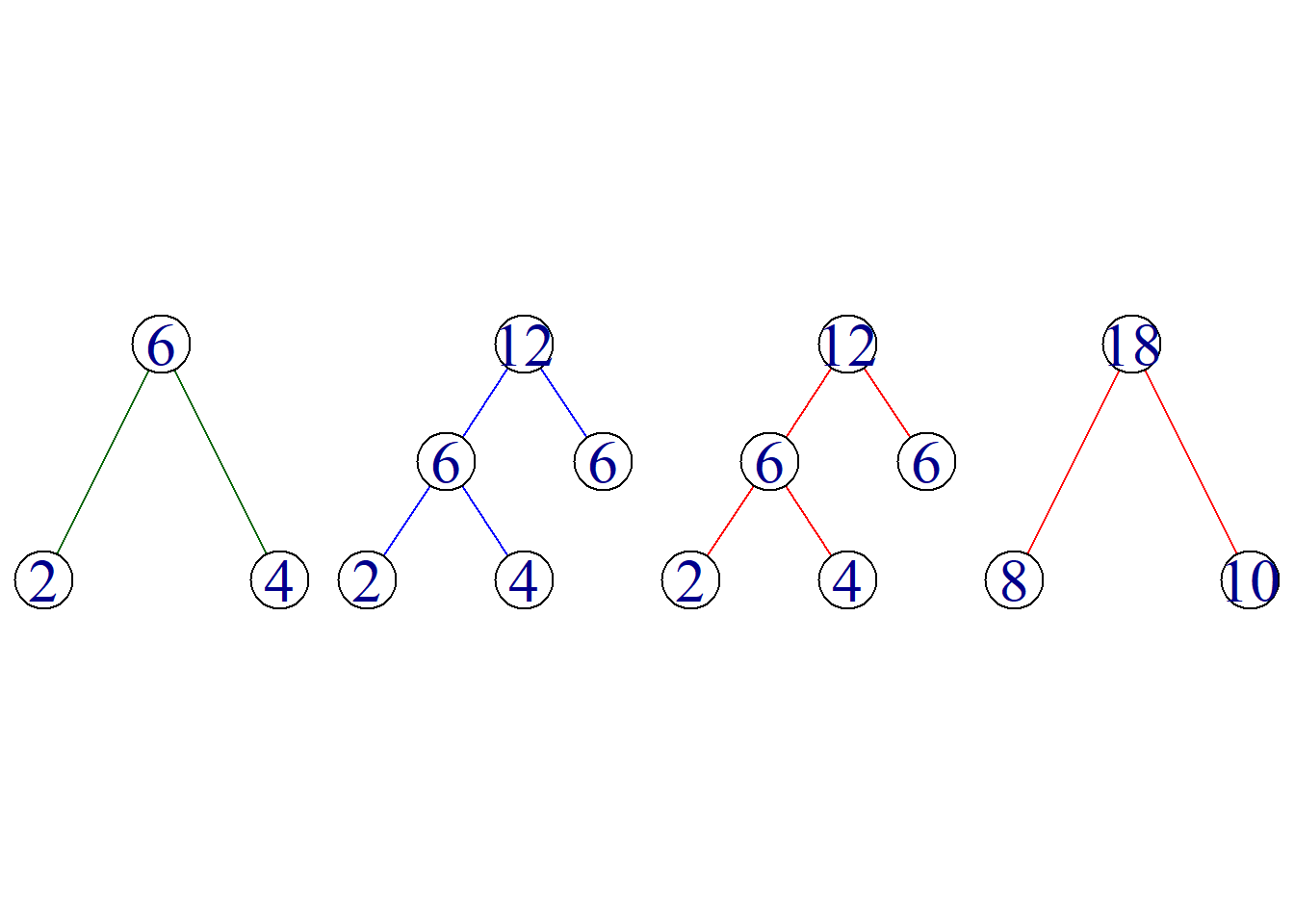
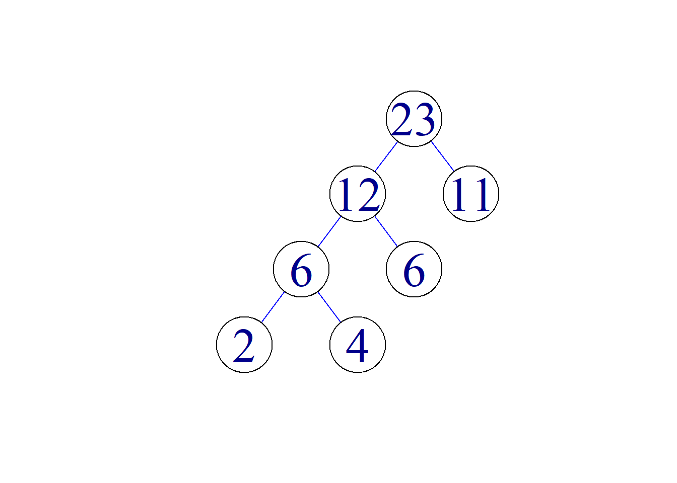
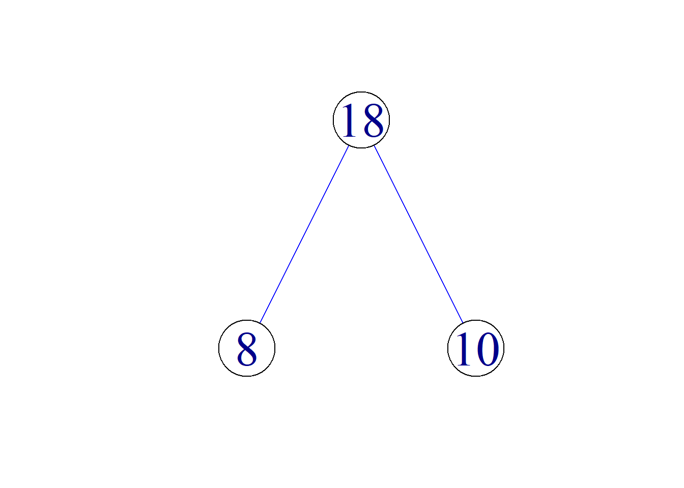
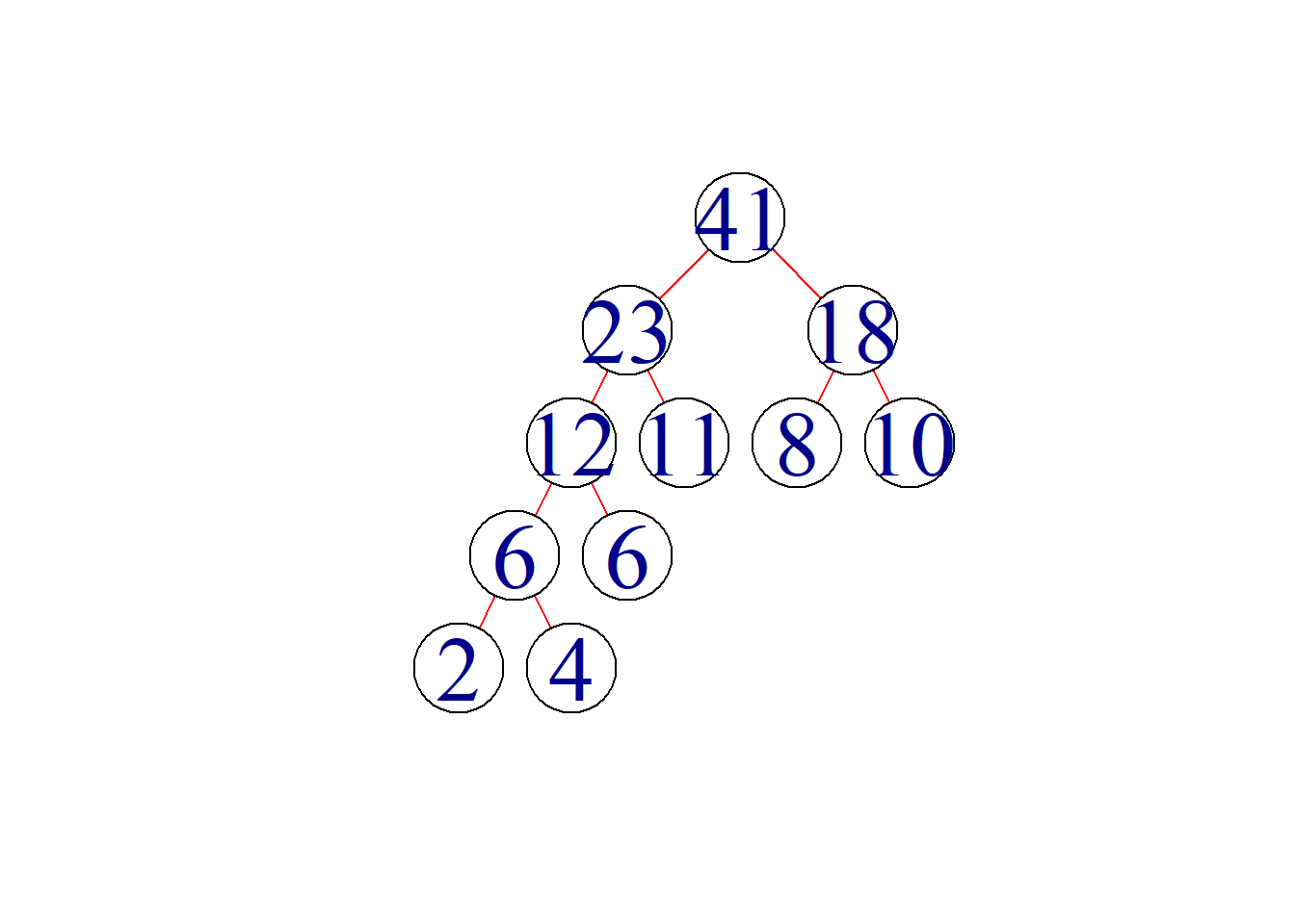
Example: Construct an optimal binary tree \(T\) with weights \(2, 4, 6, 8, 10, 11\), and find \(W(T)\).
Solution: The optimal binary tree construction process with weights \(\{2, 4, 6, 8, 10, 11\}\) is as shown in the figure.
Important applications of optimal binary trees: Huffman coding
Example: Use binary to encode \(a, b, c\) and \(d\) with equal (definite) length:
\[a{\rightarrow}00, b{\rightarrow}01, c{\rightarrow}10, d{\rightarrow}11\] Binary encoding of the character sequence \(aabba\): 0000010100.
When decoding (decoding), it corresponds to a character sequence \(aabba\), restoring the original character sequence.
\[ \begin{array}{ccccc} 00 & 00 & 01 & 01 & 00\\ a & a & b & b & a \\ \end{array} \]
Use binary to perform variable length encoding of \(a, b, c\) and \(d\):
\[a{\rightarrow}1, \, \, b{\rightarrow}00, \, \, c{\rightarrow}01, \, \, d{\rightarrow}10\]
Binary encoding of the character sequence \(aabba\): 1100001.
But when decoding:
\[ \begin{array}{ccccc} 1 & 1 & 00 & 00 & 1\\ a & a & b & b & a \\ \end{array} \] \[ \begin{array}{cccc} 1 & 10 & 00 & 01\\ a & d & b & c \\ \end{array} \]
It may correspond to two character sequences \(aabba\) or \(adbc\), resulting in ambiguity. In this case, the character sequence may not be restored after encoding. Therefore, there must be a way to determine the encoding of each character so that each character sequence corresponds to a unique binary sequence, and vice versa.
Use binary to perform variable length encoding of \(a, b, c\) and \(d\):
\[a{\rightarrow}0, \, \, b{\rightarrow}10, \, \, c{\rightarrow}110, \, \, d{\rightarrow}111\]
Binary encoding of the character sequence \(aabba\): 0010100.
When decoding, it only corresponds to one character sequence: \(aabba\).
\[ \begin{array}{ccccc} 0 & 0 & 10 & 10 & 0\\ a & a & b & b & a \\ \end{array} \]
No ambiguity occurs. This encoding is called a prefix code.
Definition: Let \(a_1a_2{\cdots}a_{n-1}a_n\) be a binary string of length \(n\), and call its substrings \(a_1, a_1a_2, {\cdots}, a_1a_2{\cdots}a_{n-1}\). The length of this binary string is \(1, 2, {\cdots}, **prefix** of n-1\).
Definition: Let \(\{\alpha_1, \alpha_2, {\cdots}, \alpha_{n-1}, \alpha_n\}\) be a set of binary strings. If any binary string in the set is not the prefix of other binary strings in the set, it is called \(\{\alpha_1, \alpha_2, {\cdots}, \alpha_{n-1}, \alpha_n\}\) is the prefix code.
For example, \(\{10, 01, 001, 1100, 00011\}\) is a prefix code.
So how to construct the prefix code? Prefix codes can be constructed through regular binary trees.
Assume \(T\) is a regular binary tree with \(t\) leaves \(v_1, v_2, {\cdots}, v_t\), then each branch point of \(T\) has two sons, and the edge leading to its left son from each branch point is marked as 0, and the edge leading to its right son is marked as 1.
Suppose \(v_i\) is any leaf of \(T\), put the binary string composed of the labels of each edge on the path from the root of the tree to the leaf \(v_i\) in order at \(v_i\), then the set of \(t\) binary strings at \(t\) leaves is the binary prefix code.
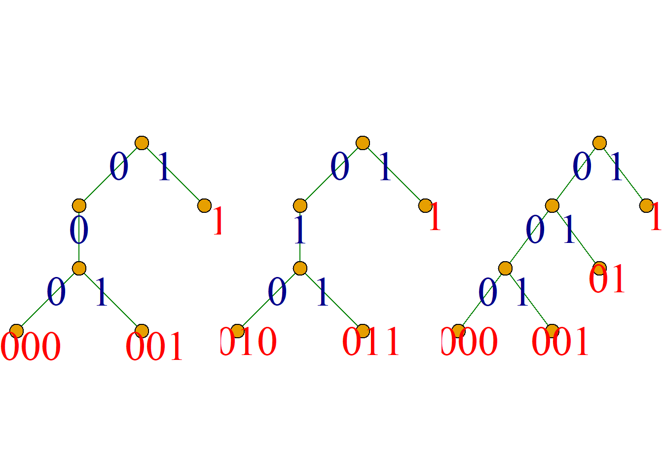
Theorem: From a given binary tree, a binary prefix code can be generated.
Theorem: From a given regular binary tree, a unique binary prefix code can be generated.
Theorem: Any prefix code corresponds to a regular binary tree.
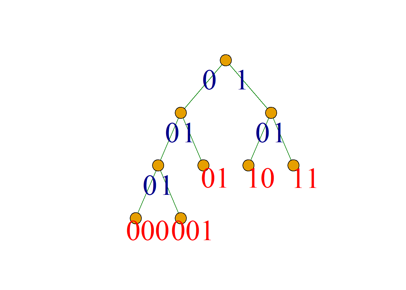
Example: For the prefix code \(\{000, 001, 01, 10, 11\}\), the corresponding regular binary tree is as follows:
Using Huffman coding can not only minimize the number of digits in the binary encoding of the character sequence, but also ensure that there will be no ambiguity during decoding. This encoding is called optimal encoding.
Example: It is known that the frequency of occurrence of letters \(A, B, C, D, E, F\) is as follows:
\[A:30\%\ B:25\%\ C:20\%\ D:10\%\ E:10\%\ F:5\%\]
Try to design an encoding scheme that minimizes the number of binary coding digits used to send 1000 letters appearing in the above ratio, and find the minimum number of digits to send.
Solution:
Construct the optimal binary tree \(T\) with weights 30, 25, 20, 10, 10, 5;
Find a prefix code (Huffman code) on \(T\).
\[\{5, 10, 10, 20, 25, 30\}{\rightarrow}\{10, 15, 20, 25, 30\}{\rightarrow}\{20, 25, 25, 30\}{\rightarrow}\{25, 30, 45\}{\rightarrow}\{45, 55\}{\rightarrow}\{100\}\]
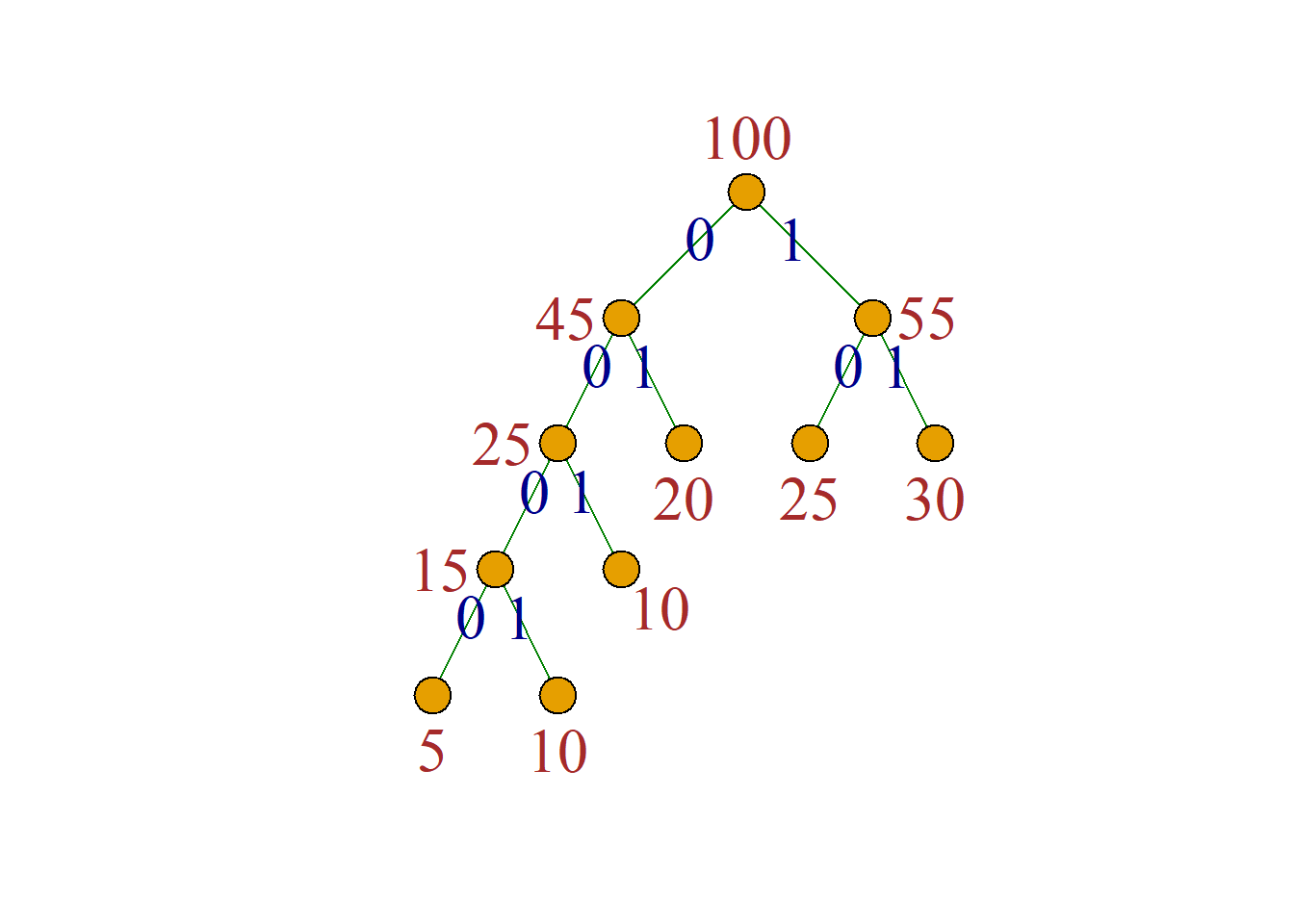
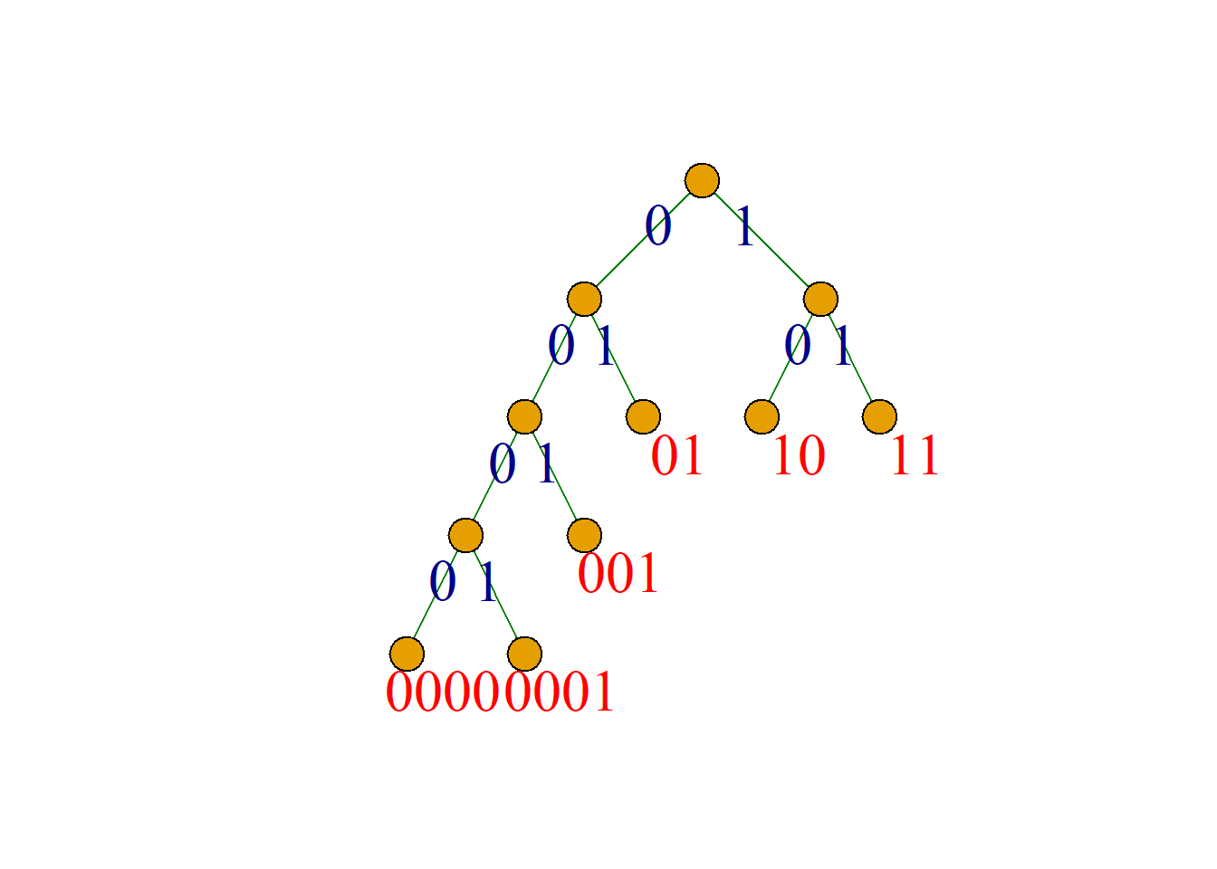
\[ \begin{array}{ccccccc} Letters & A & B & C & D & E & F\\ Coding & 11 & 10 & 01 & 001 & 0001 & 0000 \\ Sending volume & 300 & 250 & 200 & 100 & 100 & 50 \\ \end{array} \]
Number of binary digits used to send 1000 letters:
\[300{\times}2+250{\times}2+200{\times}2+100{\times}3+100{\times}4+50{\times}4=2400\] bit binary.