Graph Theory
Introduction to Graph Theory
Graph theory takes graphs as its research object and plays an important role in computer science, operations research, systems science, and mathematics.
A graph is a discrete topological structure, often used to describe and study problems in many fields.
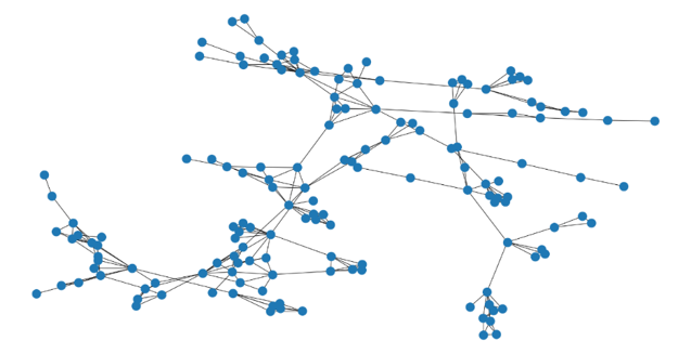
A graph in graph theory consists of a set of given vertices and edges connecting pairs of vertices, typically used to describe specific relationships between objects. Vertices represent objects, and edges between two vertices represent the various relationships between the corresponding objects.
Several classic problems in graph theory:
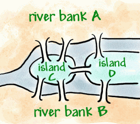
Problem 1: The Königsberg Bridge Problem (https://nrich.maths.org/2484)
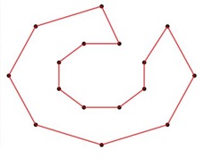
Problem 2: The Hamiltonian path problem
Problem 3: The Four color theorem
Problem 4: The Travelling salesman problem
Basic Concepts of Graphs
Definition of Graphs
Definition: Let \(A\) and \(B\) be any two sets. Define \[A\&B=\{(a, b)|a{\in}A, b{\in}B\}\] to be the unordered product of \(A\) and \(B\). \((a, b)\) is called an unordered pair.
For unordered pairs, \((a, b)=(b, a)\).
Example: Let \(A=\{a, b\}\), \(B=\{1, 2\}\), then
\[A\&B=\{(a, 1), (a, 2), (b, 1), (b, 2)\}=\{(1, a), (a, 2), (b, 1), (b, 2)\}\] \[(a, 1)=(1, a), (a, 2)=(2, a), {\cdots}\]
Graphs are classified into three types: undirected graphs, directed graphs, and mixed graphs.
Definition: An undirected graph is a triple \(G={\langle}V, E, \varphi{\rangle}\). Where:
\(V\) is a nonempty finite set whose elements are called vertices (nodes).
\(E\) is a finite set whose elements are called undirected edges.
\(\varphi\) is a mapping from the edge set \(E\) to unordered pairs of the vertex set \(V\)
(i.e., \(\varphi:E{\rightarrow}V\&V\)).
A plane diagram is commonly used to represent an undirected graph
\(G={\langle}V, E, {\varphi}{\rangle}\), called the diagram of the undirected graph.
Each vertex in \(V\) is represented by a small circle (small dot), and each edge in \(E\) is represented by a straight line or curve connecting its two endpoints.
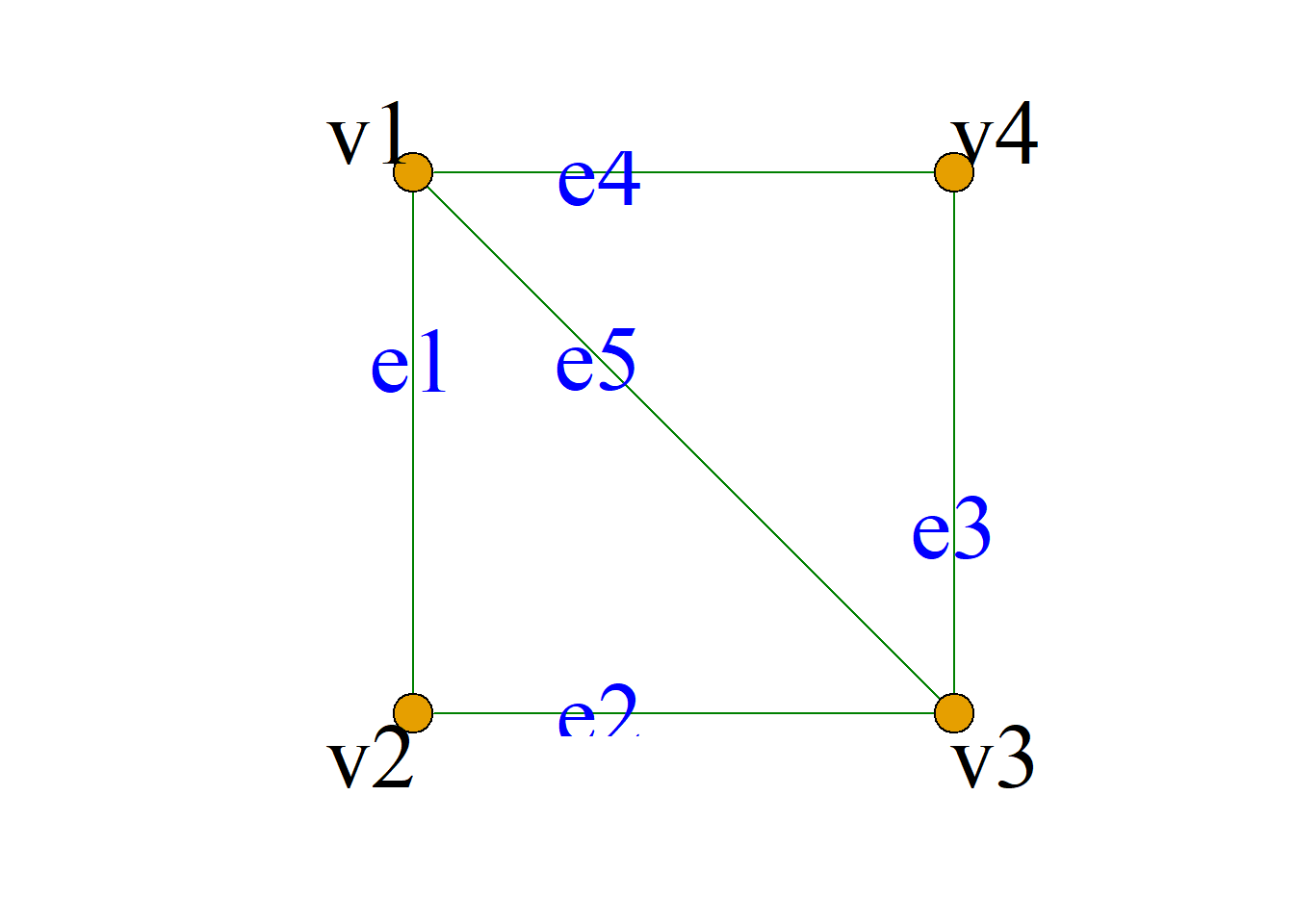
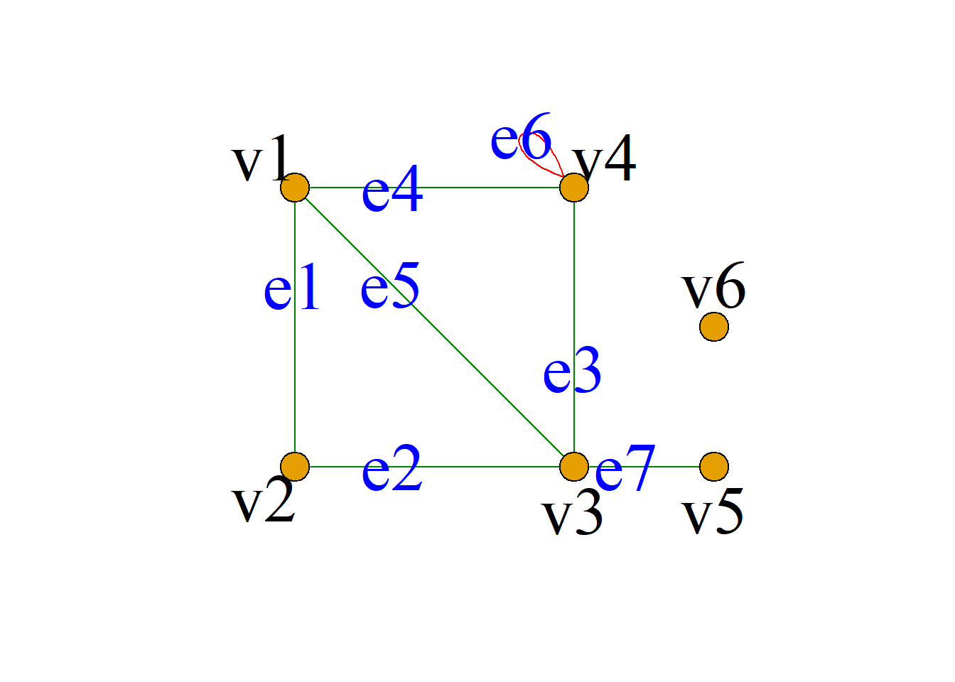
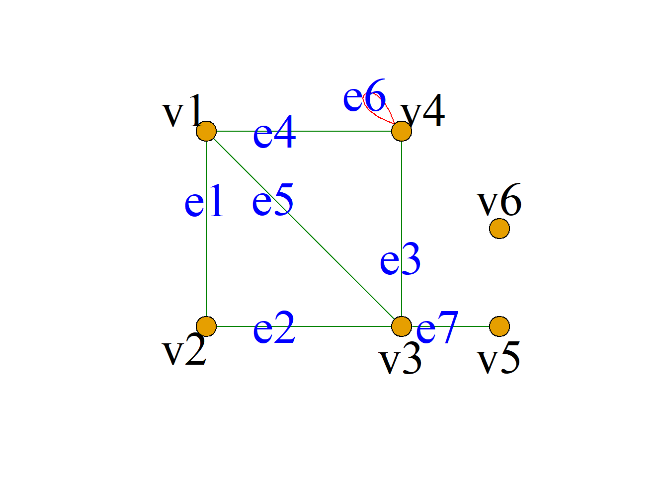
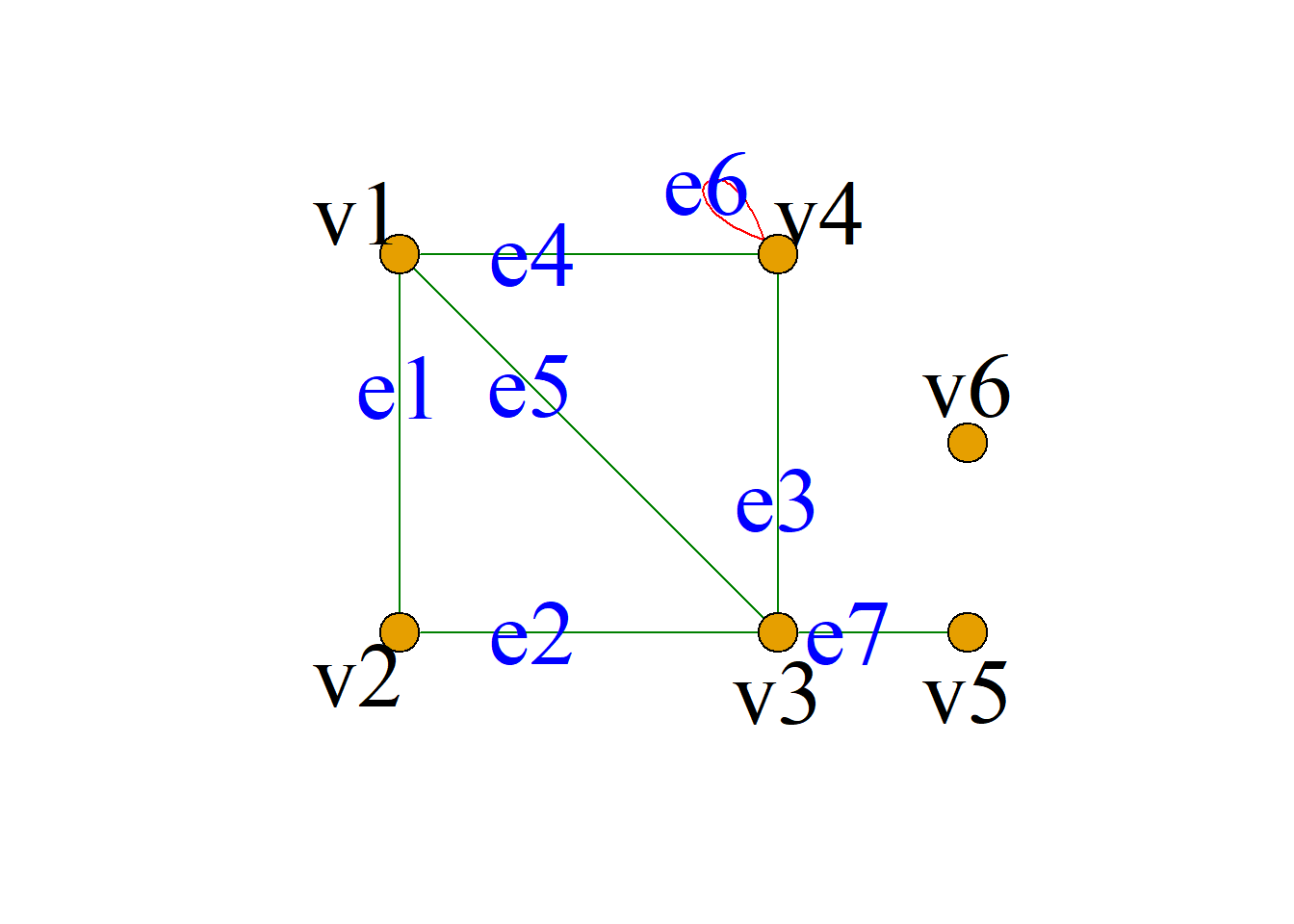
Example: Undirected graph \(G={\langle}V, E, {\varphi}{\rangle}\), where:
\[V=\{v_1, v_2, v_3, v_4, v_5, v_6\},\] \[E=\{e_1, e_2, e_3, e_4, e_5, e_6, e_7\}.\] \[{\varphi}(e_1)=(v_1, v_2),\,\,{\varphi}(e_2)=(v_2, v_3)\] \[{\varphi}(e_3)=(v_3, v_4),\,\,{\varphi}(e_4)=(v_1, v_4)\] \[{\varphi}(e_5)=(v_1, v_3),\,\,{\varphi}(e_6)=(v_4, v_4)\] \[{\varphi}(e_7)=(v_3, v_5)\] Simplified representation: \[V=\{v_1, v_2, v_3, v_4, v_5, v_6\}, \] \[E=\{(v_1, v_2), (v_2, v_3), (v_3, v_4), (v_1, v_4),\] \[(v_1, v_3), (v_4, v_4), (v_3, v_5)\}\]
Definition: A directed graph is a triple \(G={\langle}V, E, {\varphi}{\rangle}\).
Where:
\(V\) is a nonempty finite set whose elements are called vertices (nodes).
\(E\) is a finite set whose elements are called directed edges.
\({\varphi}\) is a mapping from the edge set \(E\) to ordered pairs of the vertex set \(V\)
(i.e., \({\varphi}:E{\rightarrow}V{\times}V)\).
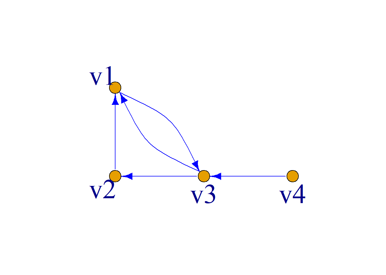
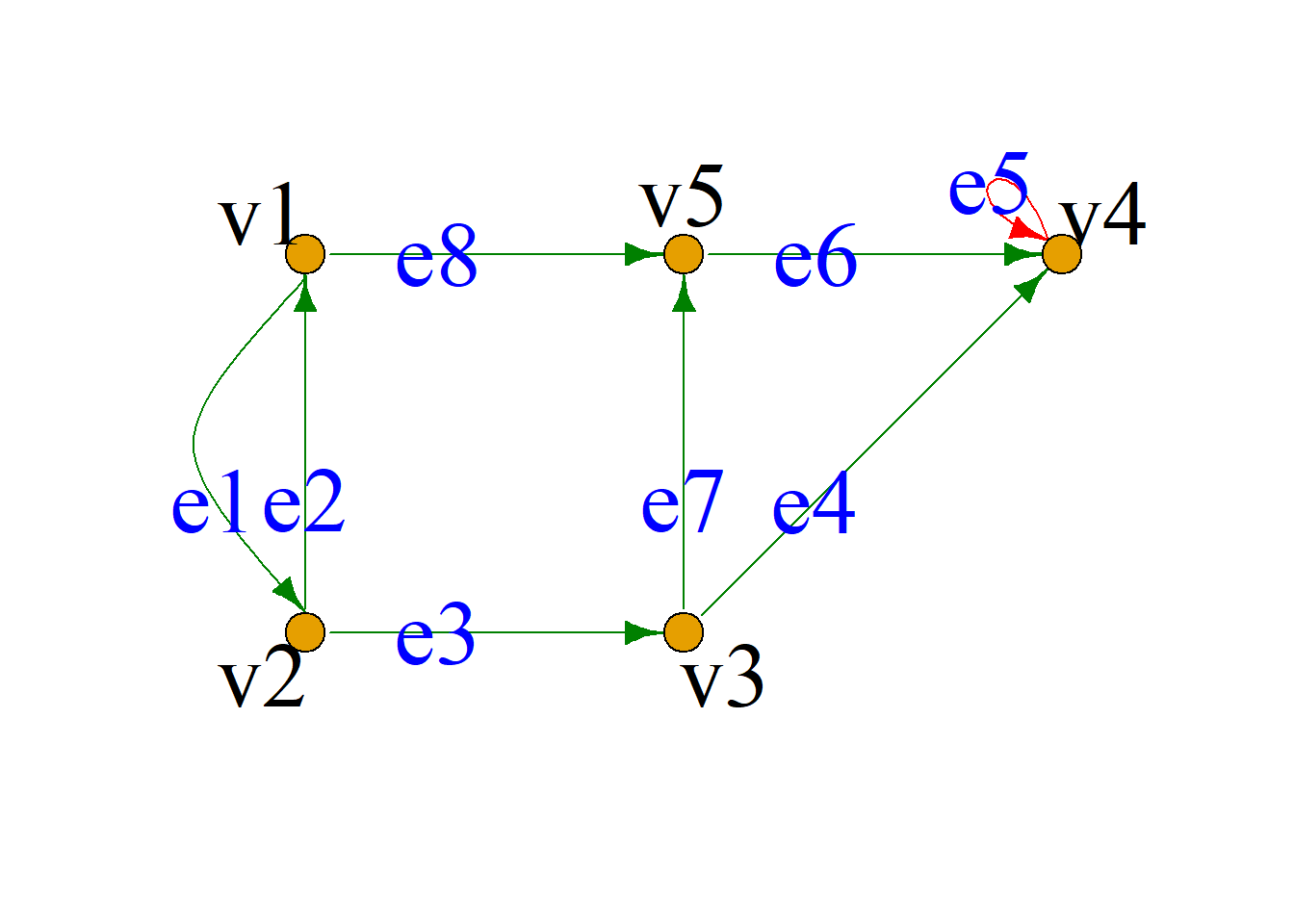
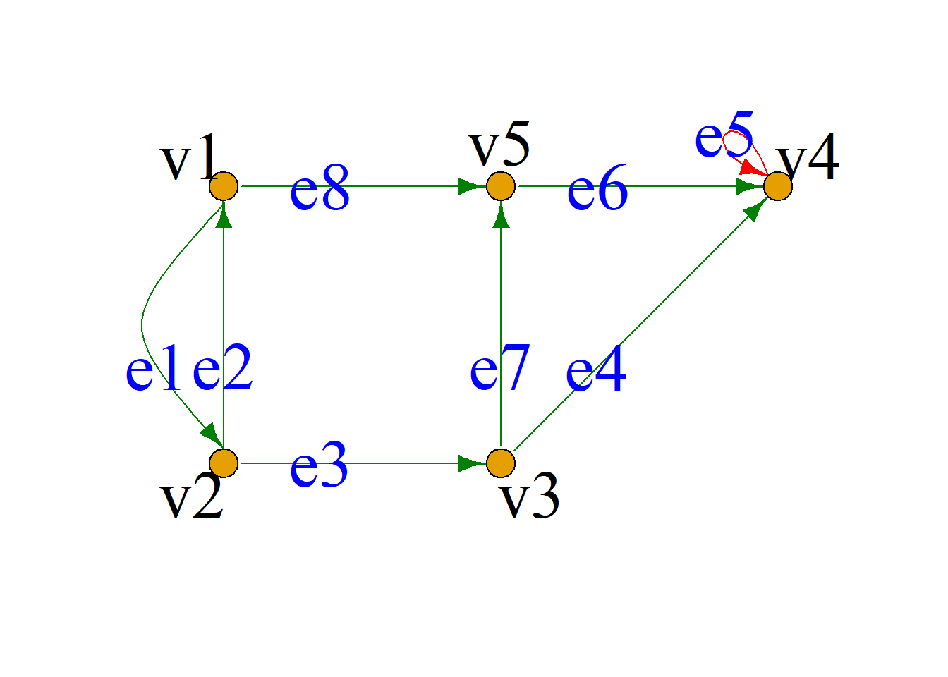
Example: Directed graph \(G={\langle}V, E, {\varphi}{\rangle}\), \(V=\{v_1, v_2, v_3, v_4, v_5\}\)
\[E=\{e_1, e_2, e_3, e_4, e_5, e_6, e_7, e_8\}\] \[{\varphi}(e_1)={\langle}v_1, v_2{\rangle},\,\,{\varphi}(e_2)={\langle}v_2, v_1{\rangle}\] \[{\varphi}(e_3)={\langle}v_2, v_3{\rangle},\,\,{\varphi}(e_4)={\langle}v_3, v_4{\rangle}\] \[{\varphi}(e_5)={\langle}v_4, v_4{\rangle},\,\,{\varphi}(e_6)={\langle}v_5, v_4{\rangle}\] \[{\varphi}(e_7)={\langle}v_3, v_5{\rangle},\,\,{\varphi}(e_8)={\langle}v_1, v_5{\rangle}\]
Simplified representation: \[V=\{v_1, v_2, v_3, v_4, v_5\}\] \[E=\{{\langle}v_2, v_1{\rangle}, {\langle}v_1, v_2{\rangle}, {\langle}v_2, v_3{\rangle}, {\langle}v_3, v_4{\rangle}, \] \[{\langle}v_4, v_4{\rangle}, {\langle}v_5, v_4{\rangle}, {\langle}v_3, v_5{\rangle}, {\langle}v_1, v_5{\rangle}\}\]
Further simplified: \(G={\langle}5, 8{\rangle}\)
Graph Terminology
Definition: In an undirected graph, if edge \(e\) is associated with the unordered pair \((v_i, v_j)\) of vertices, then vertices \(v_i\) and \(v_j\) are called the endpoints of \(e\), written \(e=(v_i, v_j)\). We say \(e\) is incident with vertices \(v_i\) and \(v_j\), and \(v_i\) and \(v_j\) are called adjacent vertices.
Two edges incident with the same vertex are called adjacent edges.
If the two endpoints of an edge are the same vertex, the edge is called a loop.
Example: \(e_1=(v_1, v_2)\); \(v_1, v_2\) are the endpoints of \(e_1\); \(e_1\) is incident with vertices \(v_1\) and \(v_2\); \(v_1\) and \(v_2\) are adjacent vertices; \(e_3\) and \(e_4\) are adjacent edges. \(e_6\) is a loop.
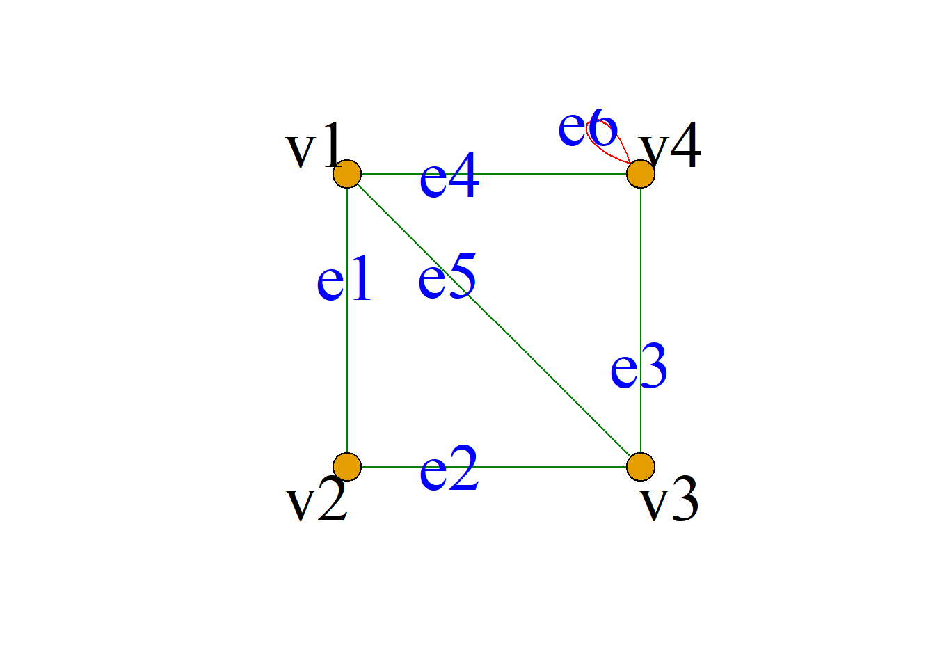
Definition: In an undirected graph, for any vertex \(v\), the number of edges incident with \(v\) is called the degree of \(v\), denoted \(d(v)\) (\(deg(v)\)). If there is a loop at vertex \(v\), the loop contributes 1 to the degree of \(v\).
Example: In graph \(G\), the degrees of the vertices are:
\[d(v_1)=3, d(v_2)=2, \] \[d(v_3)=4, d(v_4)=4, \] \[d(v_5)=1, d(v_6)=0.\]
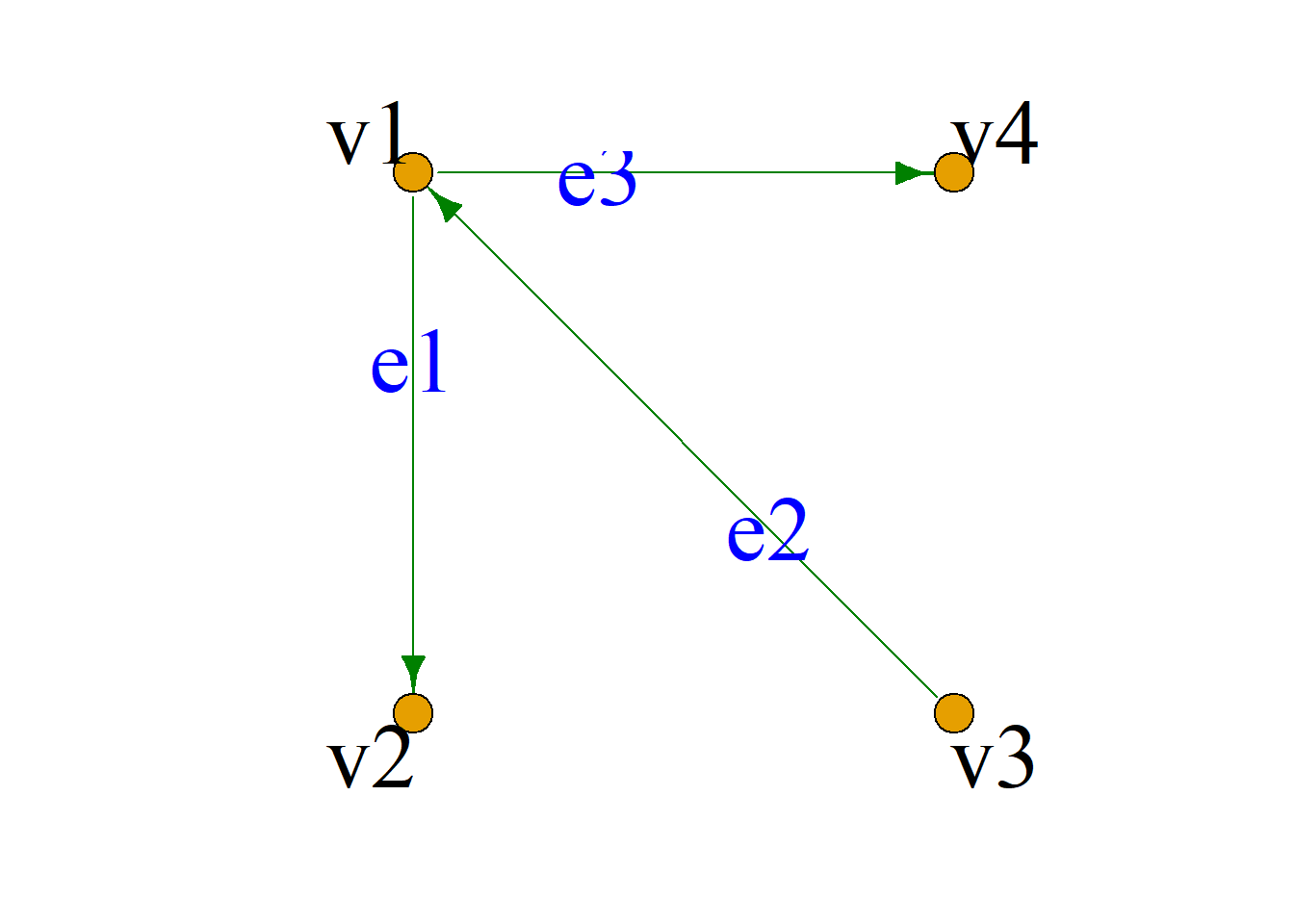
Definition: In a directed graph, if edge \(e\) is associated with the ordered pair \({\langle}v_i, v_j{\rangle}\), then \(v_i\) and \(v_j\) are called the endpoints of \(e\), written \(e={\langle}v_i, v_j{\rangle}\). \(v_i\) is called the initial vertex (tail) of \(e\), and \(v_j\) is called the terminal vertex (head) of \(e\). We say \(v_i\) is adjacent to \(v_j\), and \(v_j\) is adjacent from \(v_i\). The edge \(e\) is incident with vertices \(v_i\) and \(v_j\), and \(v_i\) and \(v_j\) are called adjacent vertices.
Two edges incident with the same vertex are called adjacent edges.
Example: \(e_2={\langle}v_3, v_1{\rangle}\); \(v_1\), \(v_3\) are the endpoints of \(e_2\); \(v_3\) is the initial vertex of \(e_2\), \(v_1\) is the terminal vertex of \(e_2\); \(e_2\) is incident with vertices \(v_1\) and \(v_3\); \(v_1\) and \(v_3\) are adjacent vertices; \(e_1\) and \(e_3\) are adjacent edges.
Definition: In a directed graph, for any vertex \(v\), the number of edges with \(v\) as initial vertex is called the out-degree of \(v\), denoted \(d^+(v)\).
The number of edges with \(v\) as terminal vertex is called the in-degree of \(v\), denoted \(d^-(v)\).
The sum of the out-degree and in-degree of a vertex is called the degree of vertex \(v\), denoted \(d(v)\).
Clearly \(d(v)=d^+(v)+d^-(v).\)
If there is a loop at vertex \(v\), the loop increases both the in-degree and out-degree of that vertex by 1 each.
Example: As shown in the graph, the degrees of the vertices are:
\[d(v_1)=d^+(v_1)+d^-(v_1)=2+1=3\] \[d(v_2)=d^+(v_2)+d^-(v_2)=2+1=3\] \[d(v_3)=d^+(v_3)+d^-(v_3)=2+1=3\] \[d(v_4)=d^+(v_4)+d^-(v_4)=1+3=4\] \[d(v_5)=d^+(v_5)+d^-(v_5)=1+2=3\]
A vertex of degree 1 is called a pendant vertex.
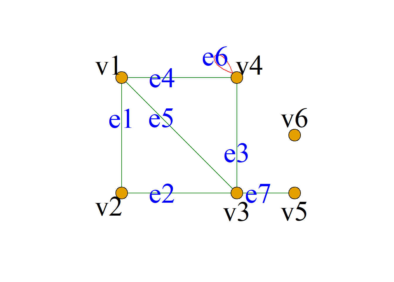
In the graph, \(v_5\) is a pendant vertex.
A vertex of degree 0 is called an isolated vertex.
In the graph, \(v_6\) is an isolated vertex.
An isolated vertex is a vertex with no incident edges.
Definition: For graph \(G={\langle}V, E{\rangle}\), define
\[\Delta(G)=max\{d(v)|v{\in}V\}\] \[\delta(G)=min\{d(v)|v{\in}V\}\]
called the maximum degree and minimum degree of graph \(G={\langle}V, E{\rangle}\), respectively. In this graph: \[\Delta(G)=4\] \[\delta(G)=0.\]
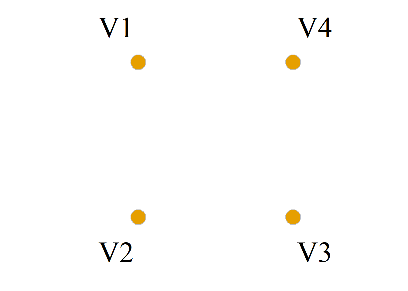
Some graphs contain only isolated vertices; such graphs are called null graphs.
In particular, a graph consisting of only a single isolated vertex is called a trivial graph.
Clearly, null graphs and trivial graphs have vertices but no edges.
Theorem (Handshaking Theorem): In any graph \(G={\langle}V, E{\rangle}\) (directed or undirected), the sum of the degrees of all vertices equals twice the number of edges:
\[\sum_{v{\in}V}d(v)=2m\] where \(m=|E|\) is the number of edges in graph \(G\).
Proof: Since each edge is incident with two vertices (a loop is incident with one vertex twice), each edge contributes 2 to the total sum of degrees. Thus \(m\) edges contribute \(2m\) degrees in total, meaning the sum of all vertex degrees is twice the number of edges.
Theorem: In any graph \(G={\langle}V, E{\rangle}\), the number of vertices with odd degree must be even.
Proof: Let \(V_1\) and \(V_2\) be the sets of vertices with even degree and odd degree in the graph, respectively. Then: \[\sum_{v{\in}V_1}d(v)+\sum_{v{\in}V_2}d(v)=\sum_{v{\in}V}d(v)=2m\] Since \(2m\) and \(\sum_{v{\in}V_1}d(v)\) are both even, \(\sum_{v{\in}V_2}d(v)\) must also be even.
Since each term in the sum \(\sum_{v{\in}V_2}d(v)\) is odd, the number of terms must be even.
Example: Does there exist an undirected graph with 6 vertices of degrees 1, 2, 3, 4, 2, 1?
Solution: No such undirected graph exists. If such a graph existed with vertex degrees 1, 2, 3, 4, 2, 1, then the number of odd-degree vertices would be 3, which is odd.
Theorem: In any directed graph \(G={\langle}V, E{\rangle}\), the sum of out-degrees of all vertices equals the sum of in-degrees of all vertices: \[\sum_{v{\in}V}d^+(v)=\sum_{v{\in}V}d^-(v)=m\] where \(m=|E|\) is the number of edges in graph \(G\).
Proof: Each directed edge has one initial vertex and one terminal vertex, so each directed edge contributes one out-degree and one in-degree. Thus \(m\) directed edges produce \(m\) out-degrees and \(m\) in-degrees.
These \(m\) out-degrees and \(m\) in-degrees are precisely the sum of out-degrees and sum of in-degrees of all vertices in the graph.
Therefore, in a directed graph, the sum of out-degrees of all vertices equals the sum of in-degrees, and both equal the number of edges.
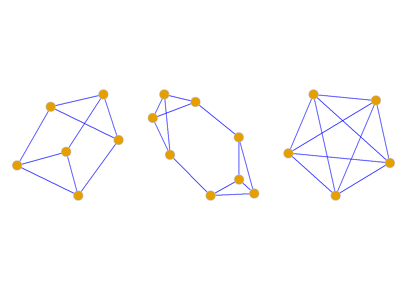
Definition: A graph in which every vertex has the same degree is called a regular graph. A regular graph in which every vertex has degree \(k\) is called a \(k\)-regular graph.
Pseudographs, Multigraphs, and Simple Graphs
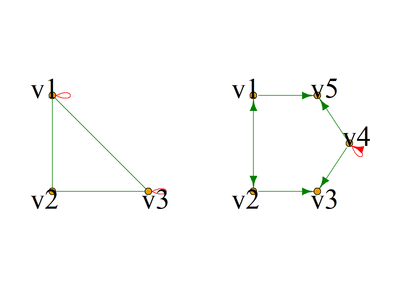
Definition: A graph containing loops is called a pseudograph.
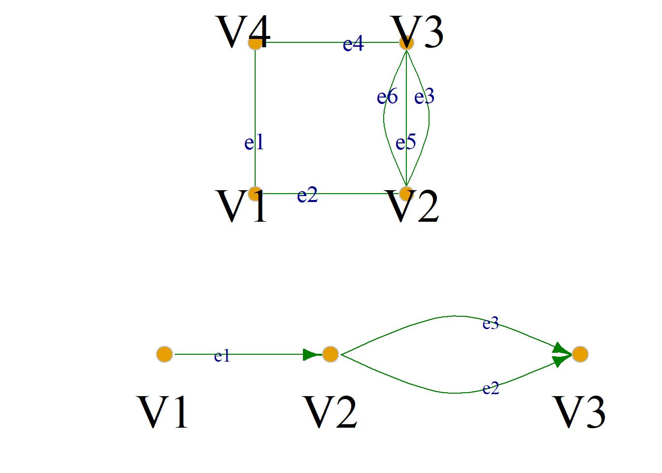
Definition: In a graph, if there are multiple edges incident with the same pair of vertices (for directed graphs, these edges must have the same initial and terminal vertices), these edges are called parallel edges or multiple edges. The number of parallel edges is called the multiplicity.
A graph containing parallel edges but no loops is called a multigraph.
The graphs on the right are all multigraphs.
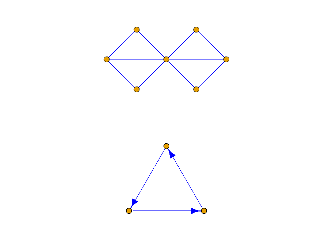
Definition: A graph containing neither parallel edges nor loops is called a simple graph.
The graphs shown are all simple graphs.
Definition: If a directed graph is a simple graph, it is called a simple directed graph.
If an undirected graph is a simple graph, it is called a simple undirected graph.
A graph containing both directed and undirected edges is called a mixed graph.
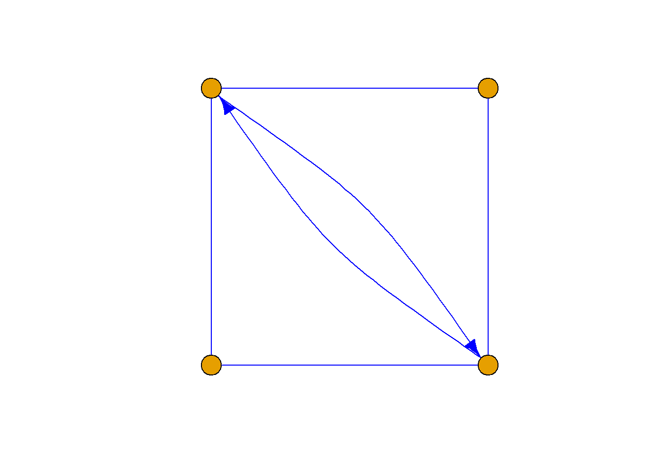
Complete Graphs
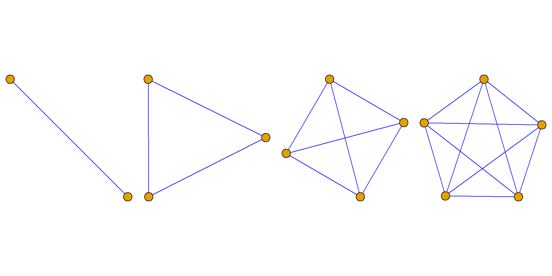
Definition: If there is exactly one undirected edge between every pair of vertices in an undirected simple graph, the graph is called an undirected complete graph. An undirected complete graph with \(n\) vertices is denoted \(K_n\).
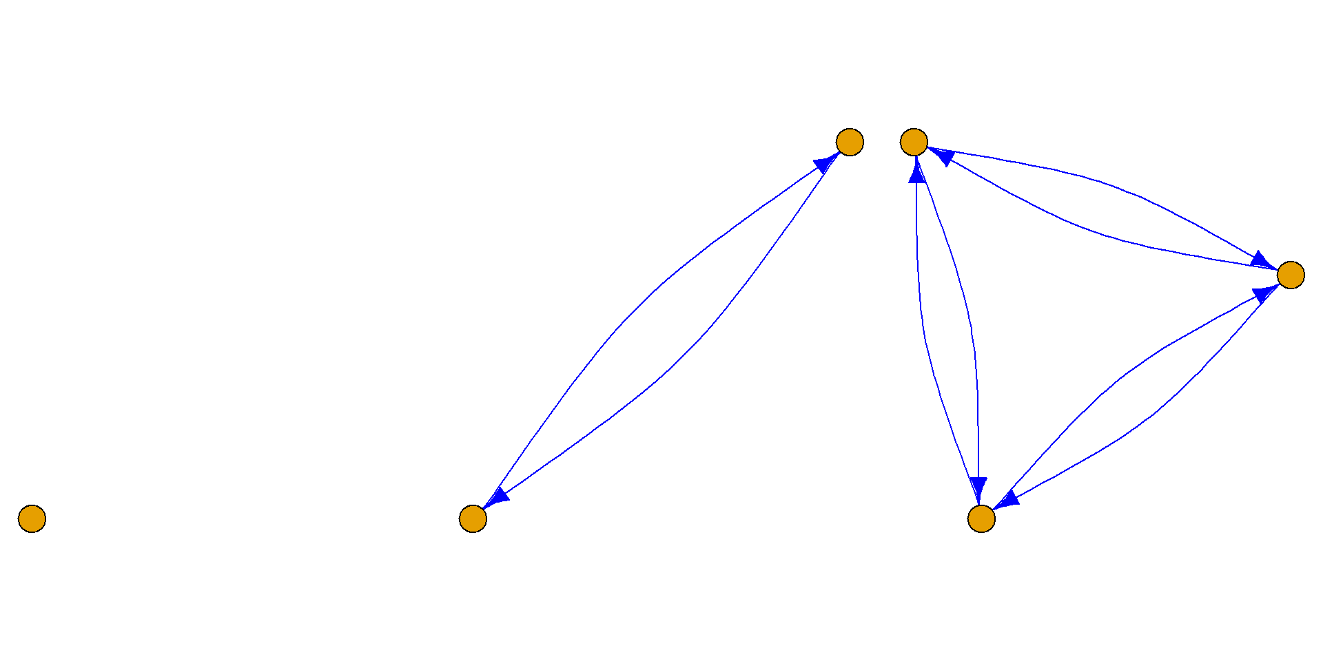
Definition: If there is exactly one pair of directed edges in opposite directions between every pair of vertices in a directed simple graph, the graph is called a directed complete graph. A directed complete graph with \(n\) vertices is denoted \(K_n\).
Theorem: For an undirected complete graph \(K_n\) with \(n\) vertices and \(m\) edges, \[m=\frac{n(n-1)}{2}\] Proof: In the undirected complete graph \(K_n\), every pair of vertices is connected by an edge. The number of ways to choose 2 vertices from \(n\) vertices is: \[C_n^2=\frac{1}{2}n(n-1)\]
Therefore, the number of edges in \(K_n\) is: \[m=\frac{n(n-1)}{2}\]
Theorem: For a directed complete graph \(K_n\) with \(n\) vertices and \(m\) edges, \(m=n(n-1)\).
Subgraphs
Definition: Let \(G={\langle}V, E{\rangle}\) and \(G^\prime={\langle}V^\prime, E^\prime{\rangle}\) be two graphs. Then:
If \(V^\prime{\subseteq}V\) and \(E^\prime{\subseteq}E\), then \(G^\prime\) is called a subgraph of \(G\), written \(G^\prime{\subseteq}G\).
If \(V^\prime{\subseteq}V\) and \(E^\prime{\subseteq}E\), but \(E^\prime{\neq}E\) or \(V^\prime{\neq}V\), then \(G^\prime\) is called a proper subgraph of \(G\), written \(G^\prime{\subset}G\).
If \(V^\prime=V\) and \(E^\prime{\subseteq}E\), then \(G^\prime\) is called a spanning subgraph of \(G\). The graph \(G\) itself and the null graph are called trivial spanning subgraphs.
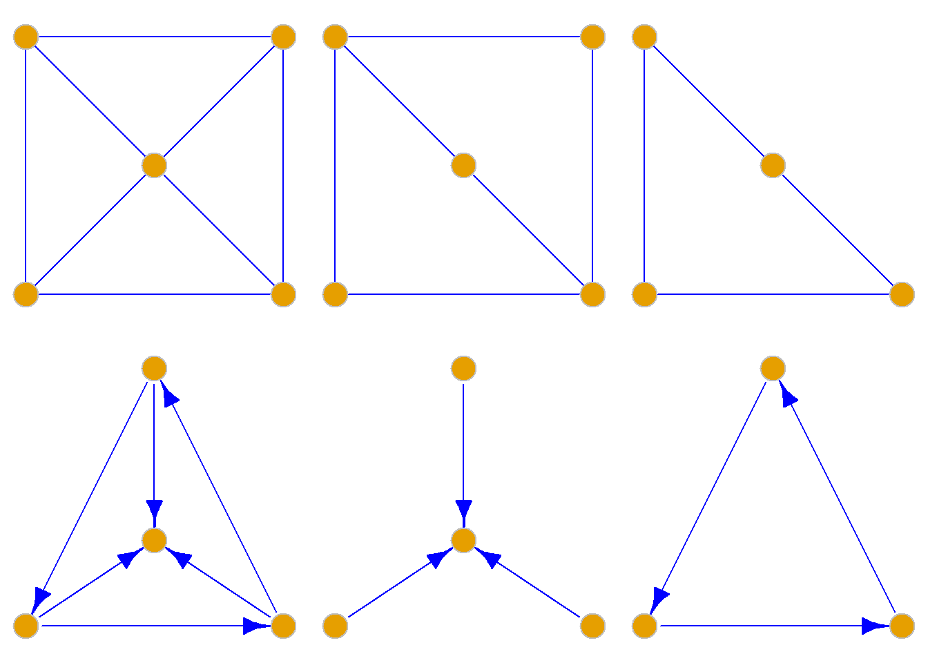
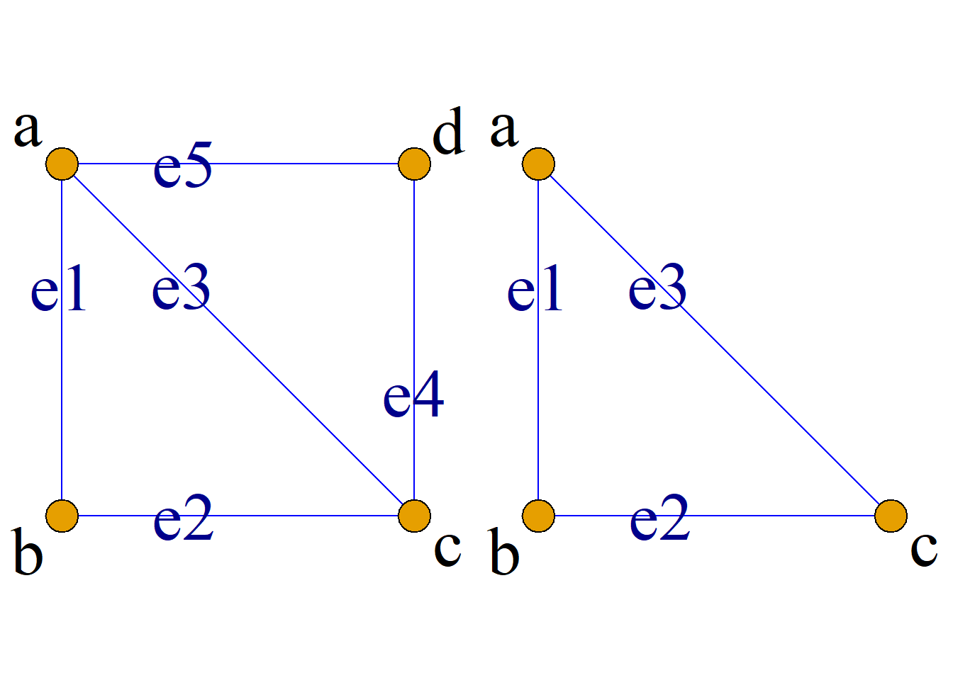
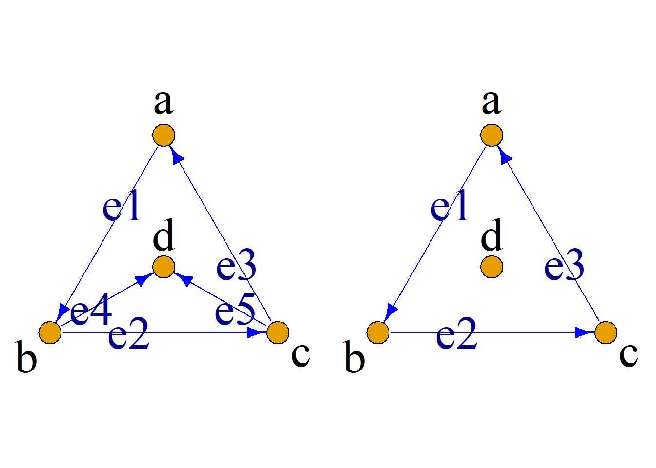
Definition: For a graph \(G={\langle}V, E{\rangle}\), let \(V^\prime{\subseteq}V\) be a nonempty subset. The graph with vertex set \(V^\prime\) and edge set consisting of all edges of \(G\) whose both endpoints are in \(V^\prime\) is called the subgraph of \(G\) induced by the vertex set \(V^\prime\), also called the vertex-induced subgraph, denoted \(G[V^\prime]\).
Example: As shown in the figure, select the subset \(V^\prime=\{a, b, c\}\)
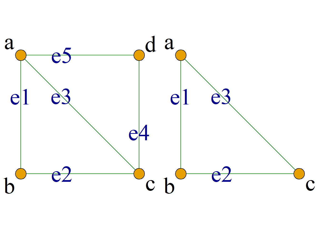
Definition: For a graph \(G={\langle}V, E{\rangle}\), let \(E^\prime\) be a nonempty subset of \(E\). The graph with edge set \(E^\prime\) and vertex set consisting of all endpoints of edges in \(E^\prime\) is called the subgraph of \(G\) induced by the edge set \(E^\prime\), also called the edge-induced subgraph, denoted \(G[E^\prime]\).
Example: As shown in the figure, select the subset \(E^\prime=\{e_1, e_2, e_3\}\)
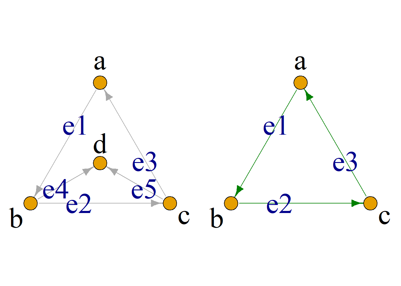
Representations of several types of induced subgraphs:
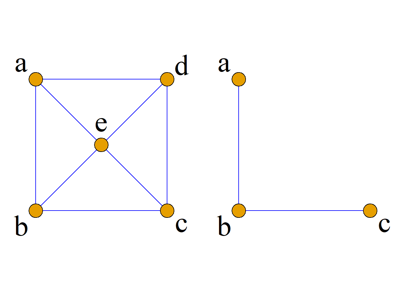
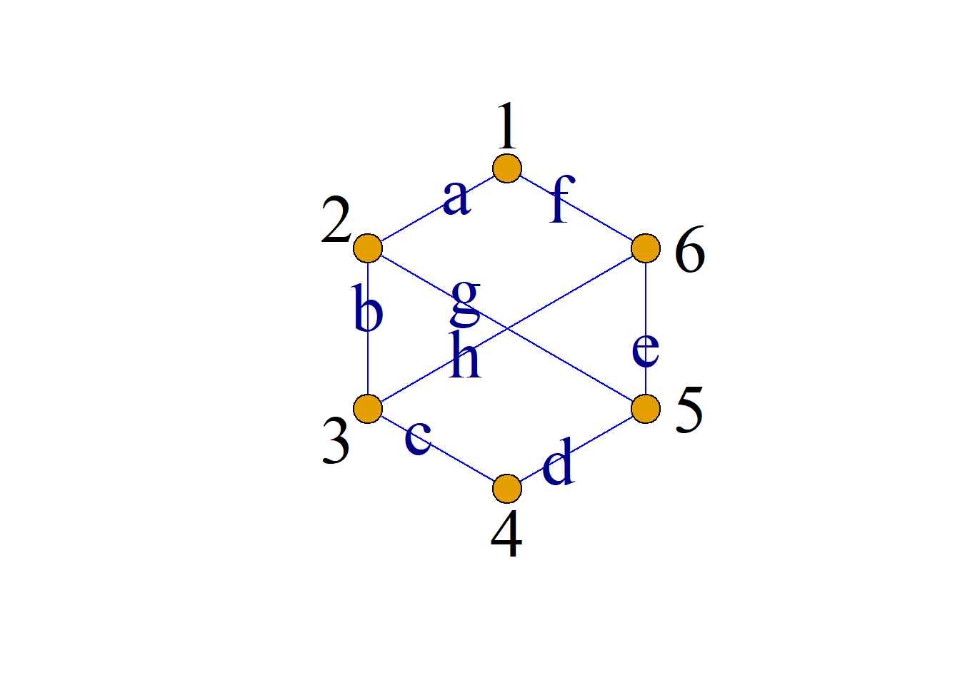
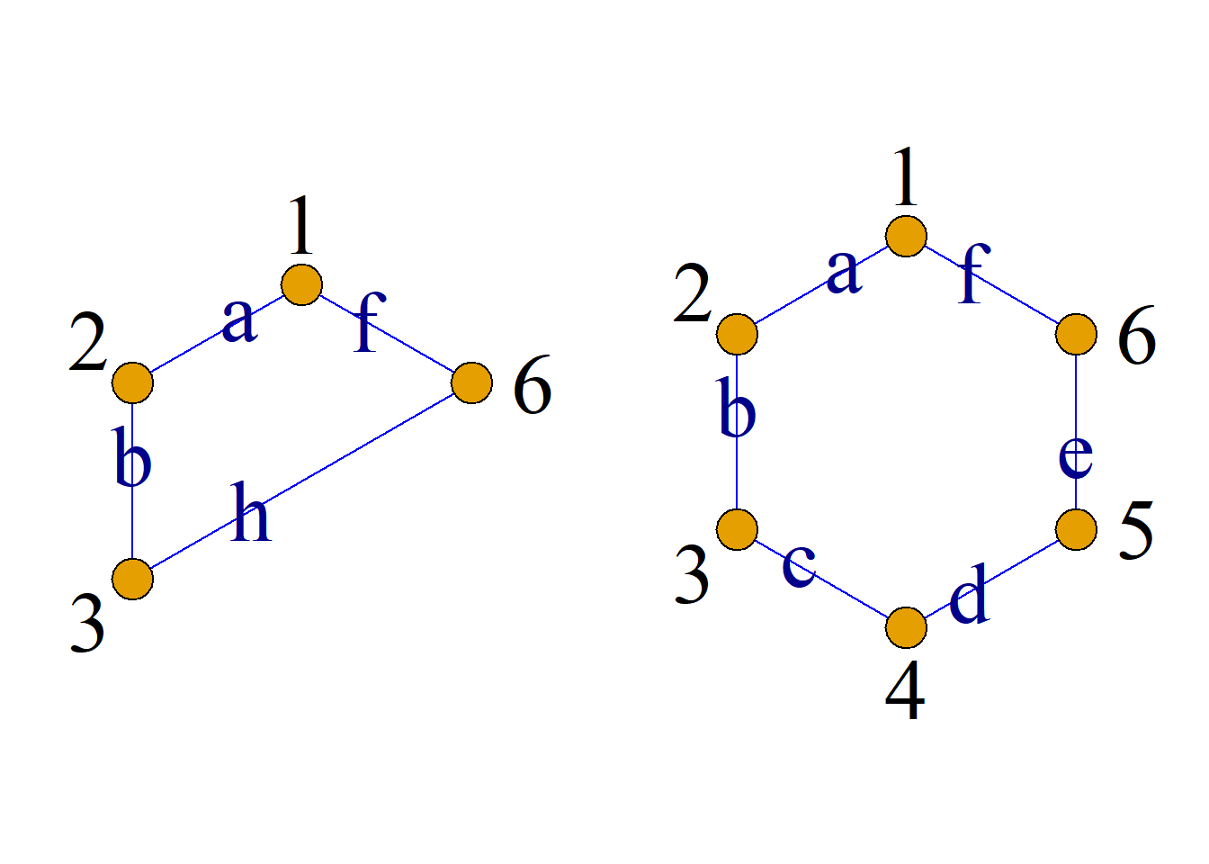
For a graph \(G={\langle}V, E{\rangle}\) and \(V^\prime{\subseteq}V\), deleting from \(G\) all vertices in \(V^\prime\) and all edges incident to those vertices yields a subgraph denoted \(G-V^\prime\), which is actually the induced subgraph \(G[V-V^\prime]\).
In particular, if \(V^\prime=\{v\}\), it is simply written as \(G-v\).
Example: \(G-\{d, e\}\).
For a graph \(G={\langle}V, E{\rangle}\) and \(E^\prime{\subseteq}E\), deleting from \(G\) all edges in \(E^\prime\) yields a subgraph of \(G\) denoted \(G-E^\prime\), which is actually the spanning subgraph of \(G\) with vertex set \(V\) and edge set \(E-E^\prime\).
In particular, if \(E^\prime=\{e\}\), it is simply written as \(G-e\).
Complement Graph
Definition: Let \(G^\prime={\langle}V^\prime, E^\prime{\rangle}\) be a subgraph of graph \(G={\langle}V, E{\rangle}\).
Given another graph \(G^{\prime\prime}={\langle}V^{\prime\prime}, E^{\prime\prime}{\rangle}\), if \(E^{\prime\prime}=E-E^\prime\) and \(V^{\prime\prime}\) is the set of vertices incident to edges in \(E^{\prime\prime}\) plus any isolated vertices present in \(G\) but not in \(G^\prime\), then \(G^{\prime\prime}\) is called the complement of subgraph \(G^\prime\) with respect to graph \(G\), denoted \(G^{\prime\prime}=G-G^\prime\).
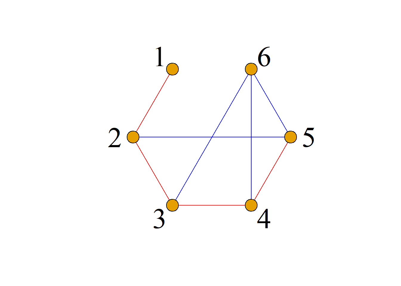
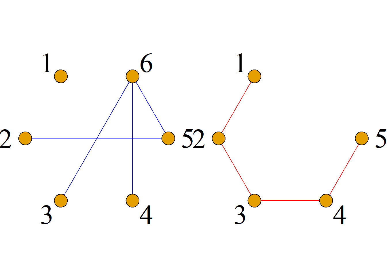
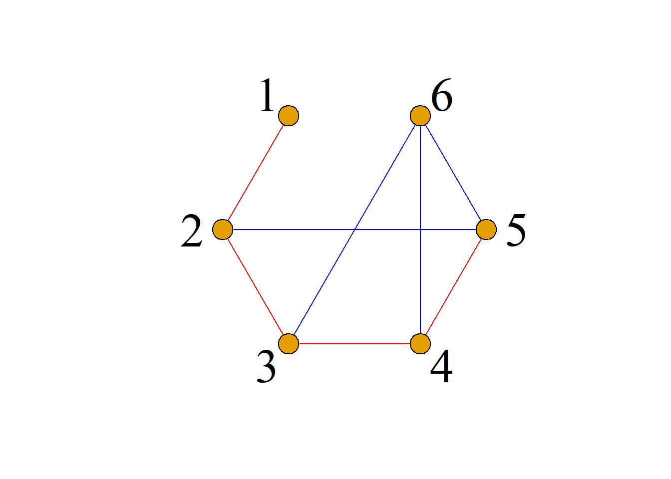
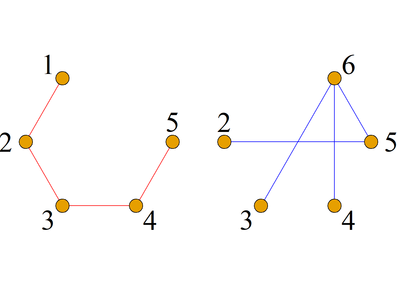
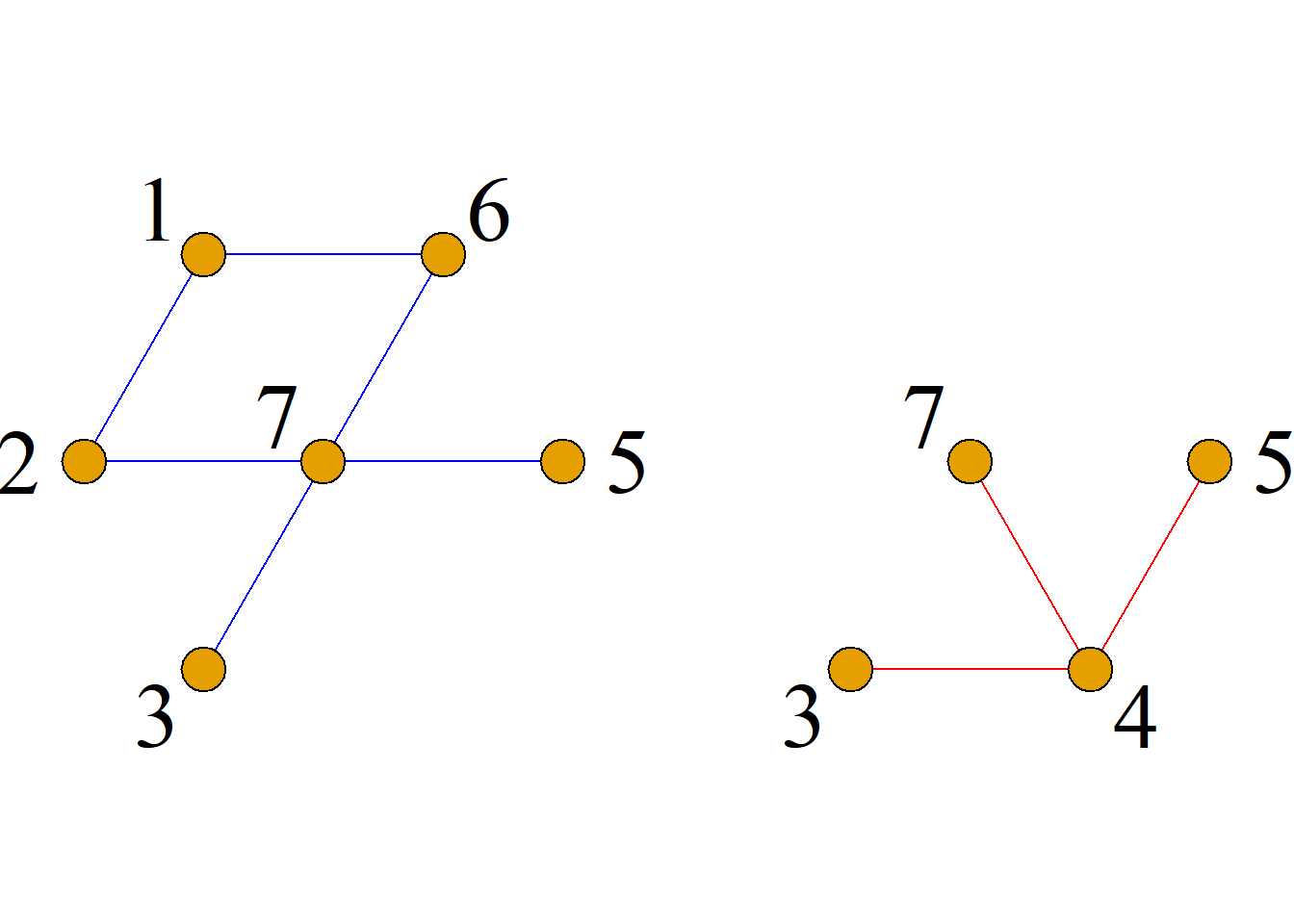
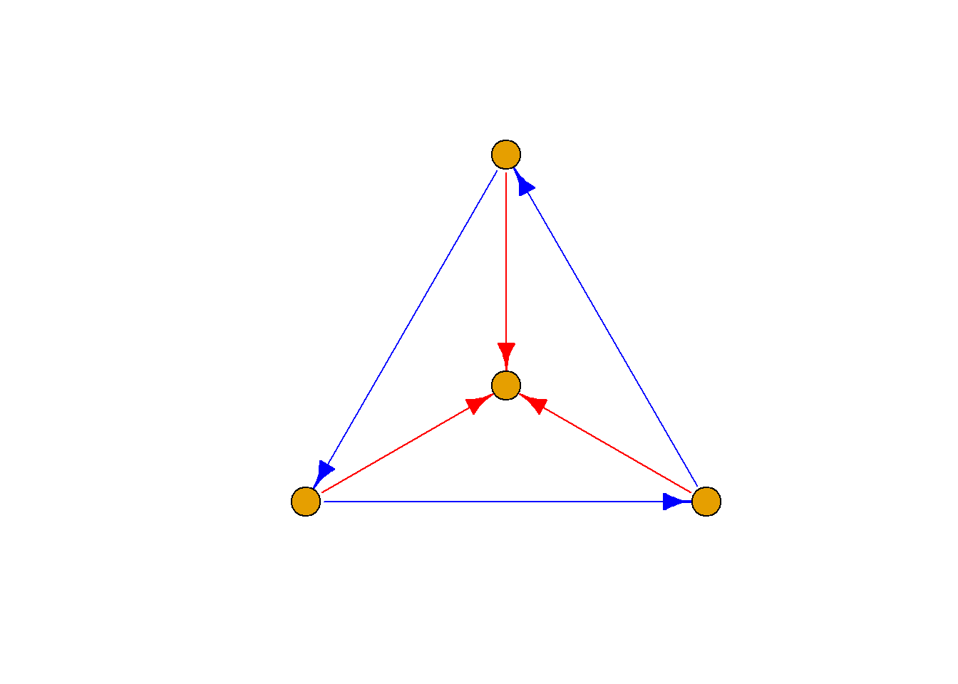
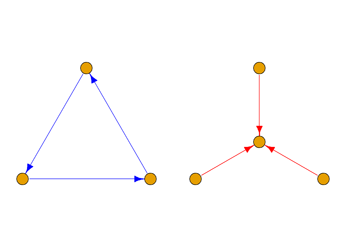
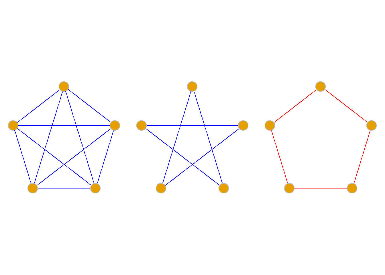
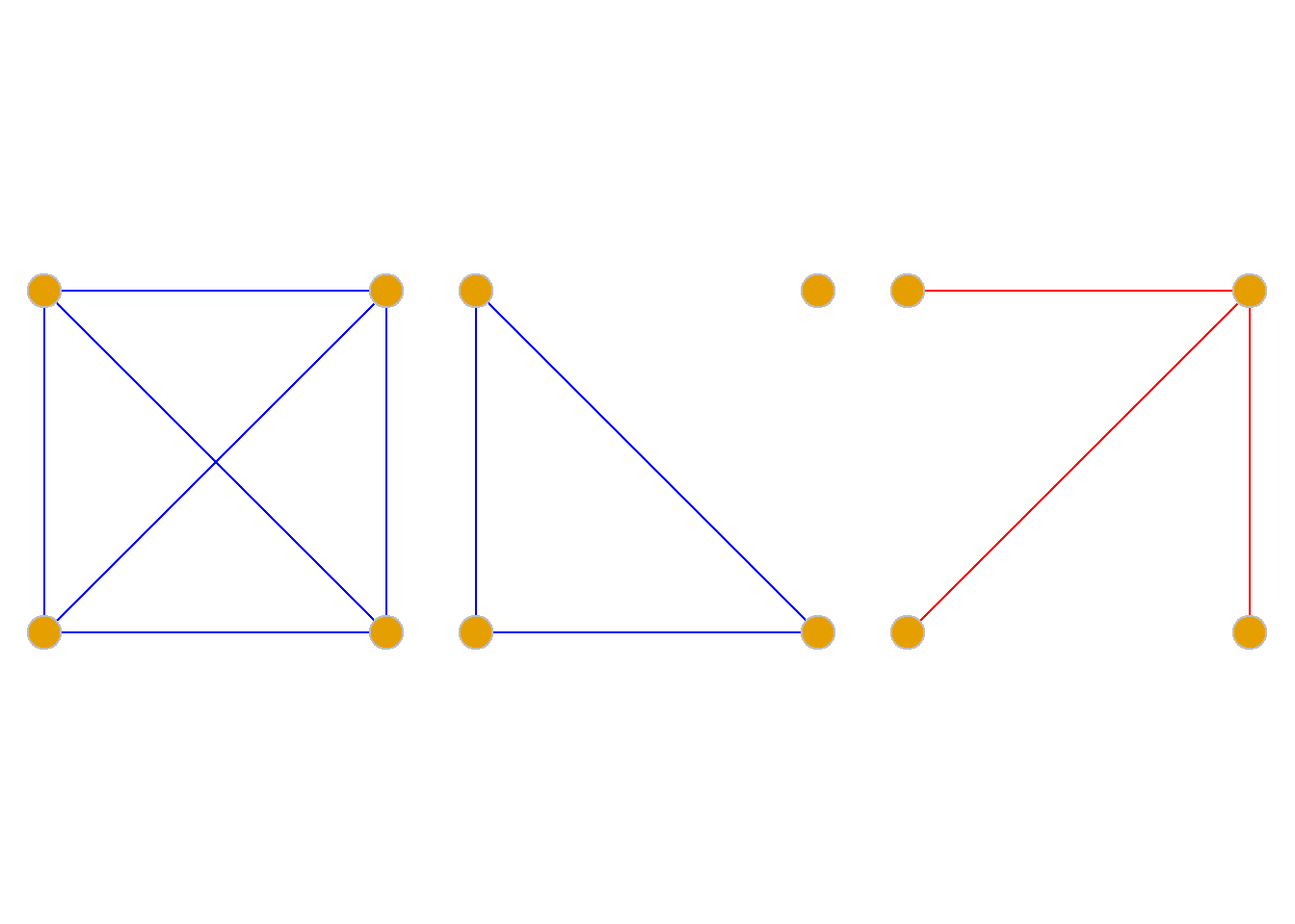
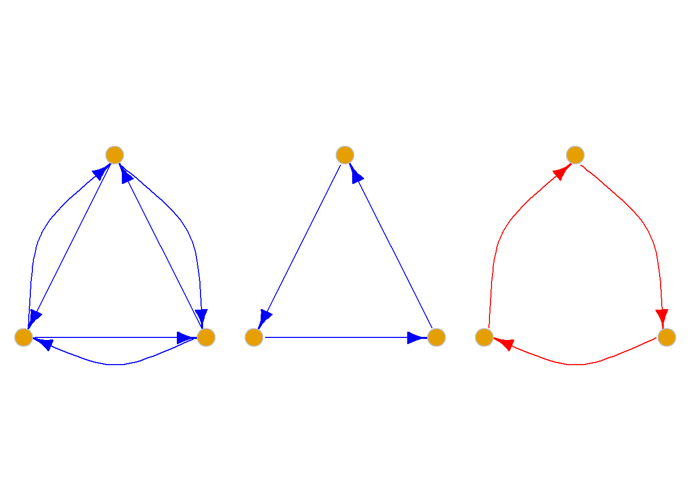
Definition: Let \(G={\langle}V, E{\rangle}\) be a simple graph with \(n\) vertices. The graph with vertex set \(V\) and edge set consisting of all edges that would need to be added to make \(G\) the complete graph \(K_n\) is called the complement of \(G\) with respect to \(K_n\), simply called the complement graph of \(G\), denoted \(\bar{G}\).
Clearly, \(G\) and \(\bar{G}\) are complementary.
Graph Isomorphism
Definition: Given undirected graphs \(G={\langle}V, E{\rangle}\) and \(G^\prime={\langle}V^\prime, E^\prime{\rangle}\), if there exists a bijection \(f:V{\rightarrow}V^\prime\) such that for any \[e=(v_i, v_j){\in}E{\,\,\Leftrightarrow\,\, }e^\prime=(f(v_i), f(v_j)){\in}E^\prime, \]then \(G\) and \(G^\prime\) are called isomorphic, written \(G{\cong}G^\prime.\) The function \(f\) is called an isomorphism from \(G\) to \(G^\prime\).
Definition: Given directed graphs \(G={\langle}V, E{\rangle}\) and \(G^\prime={\langle}V^\prime, E^\prime{\rangle}\), if there exists a bijection \(f:V{\rightarrow}V^\prime\) such that for any \[e={\langle}v_i, v_j{\rangle}{\in}E\,\,{\Leftrightarrow}\,\,e^\prime={\langle}f(v_i), f(v_j){\rangle}{\in}E^\prime, \]then \(G\) and \(G^\prime\) are called isomorphic, written \(G{\cong}G^\prime\). The function \(f\) is called an isomorphism from \(G\) to \(G^\prime\).
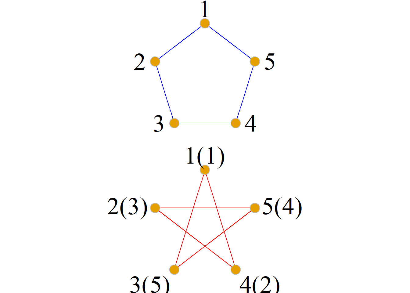
Two graphs are isomorphic if and only if there is a one-to-one correspondence between their vertices and edges that preserves the incidence relation; for directed graphs, this correspondence must also preserve the direction of edges.
In fact, the intuitive meaning of graph isomorphism is that one graph can be superimposed on the other through rotation, translation, stretching, and other deformations.
Graph isomorphism is a very important problem in graph theory.
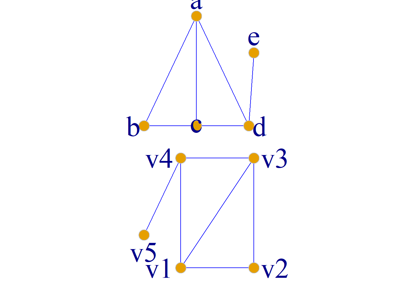
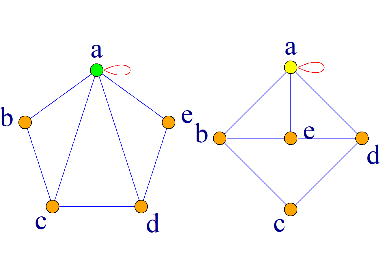
Graphs \(G_1\) and \(G_2\) are isomorphic, since the following bijection \(f\) can be established: \[\{a, b, c, d, e\}{\leftrightarrow}\{v_3, v_2, v_1, v_4, v_5\}\] \[(a, b){\leftrightarrow}(v_3, v_2)\] \[(a, c){\leftrightarrow}(v_1, v_3)\] \[(a, d){\leftrightarrow}(v_3, v_4)\] \[(b, c){\leftrightarrow}(v_2, v_1)\] \[(c, d){\leftrightarrow}(v_1, v_4)\] \[(d, e){\leftrightarrow}(v_4, v_5)\]
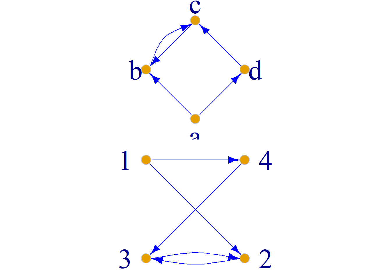
Example: (a) and (b) are isomorphic, since there exists a bijection \(f\): \[\{a, b, c, d\}{\leftrightarrow}\{1, 2, 3, 4\}\] \[{\langle}a, b{\rangle}{\leftrightarrow}{\langle}1, 2{\rangle}\] \[{\langle}a, d{\rangle}{\leftrightarrow}{\langle}1, 4{\rangle}\] \[{\langle}b, c{\rangle}{\leftrightarrow}{\langle}2, 3{\rangle}\] \[{\langle}c, b{\rangle}{\leftrightarrow}{\langle}3, 2{\rangle}\] \[{\langle}d, c{\rangle}{\leftrightarrow}{\langle}4, 3{\rangle}\]
Two isomorphic graphs have the following properties:
The two graphs have the same number of vertices.
The two graphs have the same number of edges.
The two graphs have the same number of vertices of each degree.
Let \(v{\in}V\), \(f(v)=u{\in}V^\prime\), then \(d(v)=d(u)\)
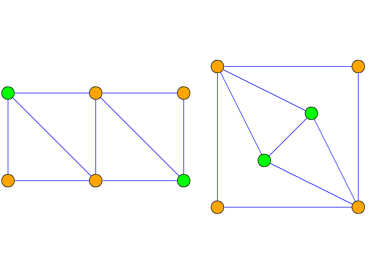
These four properties are necessary but not sufficient conditions for two graphs to be isomorphic. That is, isomorphic graphs must satisfy all these properties; if any one of these properties is not satisfied, the two graphs are definitely not isomorphic.
Graph Connectivity
Walks and Cycles
Definition: Given a graph \(G={\langle}V, E{\rangle}\), let \(v_0, v_1, {\cdots}, v_k{\in}V, e_1, e_2, {\cdots}, e_k{\in}E\), where each \(e_i|(i=1, 2, {\cdots})\) has \(v_{i-1}\) and \({v_i}\) as its endpoints (for a directed graph, \(v_{i-1}\) is the tail and \(v_i\) is the head of \(e_i\)). The alternating sequence of vertices and edges \(v_0e_1v_1e_2{\cdots}e_kv_k\) is called a walk or path from vertex \(v_0\) to vertex \(v_k\).
\(v_0\) and \(v_k\) are called the origin and terminus of the walk, respectively; the number of edges \(k\) is called the length of the walk.
When \(v_0=v_k\), the walk is called a circuit or cycle.
If all edges in a walk are distinct, the walk is called a simple walk or simple path. If all edges in a circuit are distinct, the circuit is called a simple circuit or simple cycle.
If all vertices in a walk are distinct, the walk is called an elementary path or simple path.
If all vertices in a circuit are distinct (except the origin and terminus), the circuit is called an elementary circuit or elementary cycle.
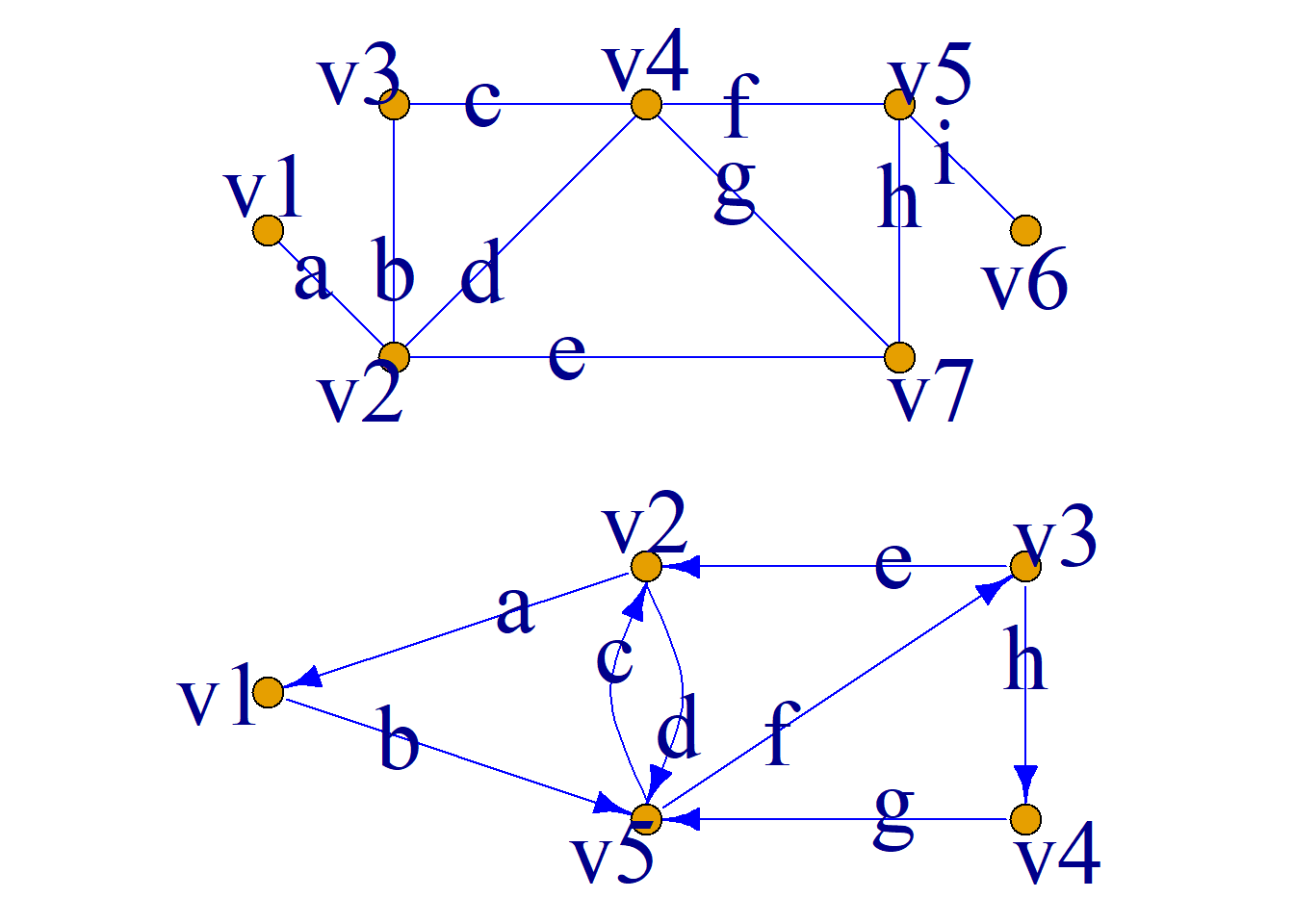
Example: As shown in the figure.
In (a), \(v_1av_2bv_3cv_4dv_2ev_7\) is a simple walk of length 5,
\(v_1av_2ev_7hv_5iv_6\) is an elementary path of length 4.
In (b), \(v_1bv_5cv_2dv_5fv_3ev_2av_1\) is a simple circuit of length 6,
\(v_5cv_2dv_5\) is an elementary circuit of length 2.
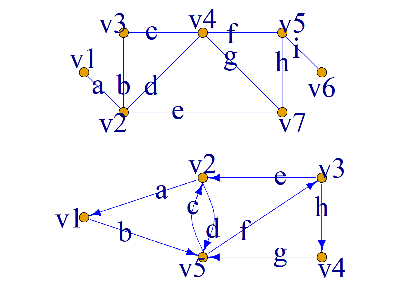
In (a), the simple walk \(v_1av_2bv_3cv_4dv_2ev_7\) can be represented by the edge sequence \(abcde\) or by the vertex sequence \(v_1v_2v_3v_4v_2v_7\).
In (b), the simple circuit \(v_1bv_5cv_2dv_5fv_3ev_2av_1\) can be represented by the edge sequence \(bcdfea\) or by the vertex sequence \(v_1v_5v_2v_5v_3v_2v_1\).
Theorem: In a graph \(G\), if there exists a walk from vertex \(v_i\) to vertex \(v_j\), then there exists an elementary path from \(v_i\) to \(v_j\).
Theorem: In a graph \(G\), if there exists a circuit from vertex \(v_i\) to vertex \(v_i\), then there exists an elementary circuit from \(v_i\) to \(v_i\).
Theorem: In a graph with \(n\) vertices:
The length of any elementary path is at most \(n-1\).
The length of any elementary circuit is at most \(n\).
Graph Connectivity
Definition: Given a graph \(G={\langle}V, E{\rangle}\), let \(v_i\) and \(v_j\) be two vertices in \(G\). If there exists a walk from \(v_i\) to \(v_j\), we say that \(v_j\) is reachable from \(v_i\).
By convention, every vertex in \(G\) is always reachable from itself.
For an undirected graph, if \(v_i\) is reachable from \(v_j\), then \(v_j\) is also reachable from \(v_i\); that is, vertices \(v_i\) and \(v_j\) are mutually reachable.
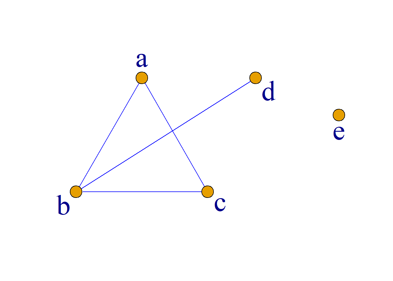
Example: As shown in graph \(G\), \(a\) is reachable from \(d\), \(d\) is reachable from \(a\), so \(a\) and \(d\) are mutually reachable. \(b\) is not reachable from \(e\).
For a directed graph, if \(v_j\) is reachable from \(v_i\), it does not necessarily mean that \(v_i\) is reachable from \(v_j\).
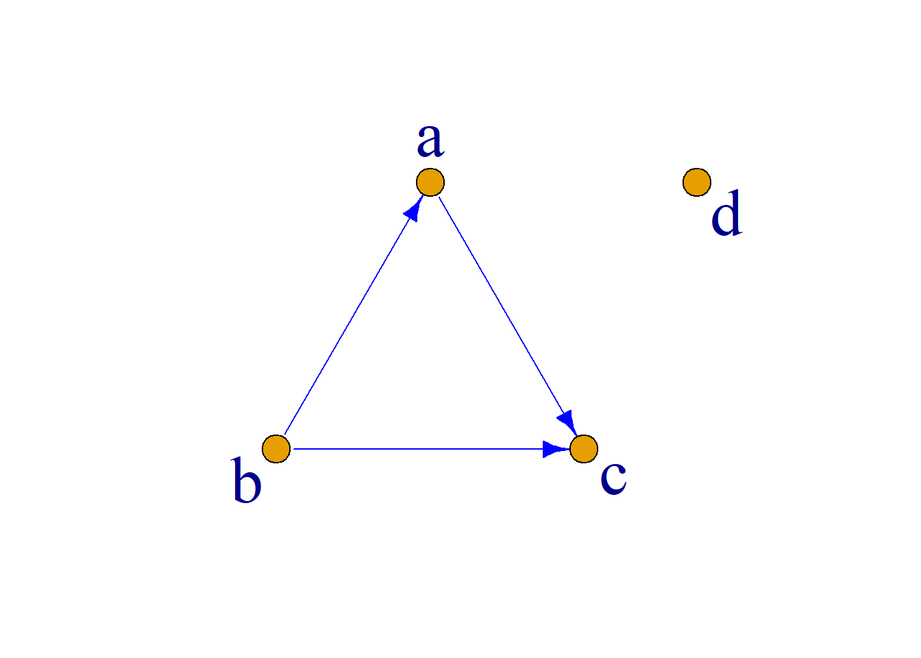
Example: As shown in graph \(G_1\), \(c\) is reachable from \(a\), but \(a\) is not reachable from \(c\).
Definition: For any two vertices \(v_i\) and \(v_j\) in graph \(G={\langle}V, E{\rangle}\), define the distance \(d[v_i, v_j]\) from \(v_i\) to \(v_j\) as follows: \[ d[v_i, v_j]= \begin{cases} 0 & i=j \\ \infty & i{\neq}j, v_i\text{ cannot reach }v_j \\ l & i{\neq}j, v_i\text{ can reach }v_j \\ \end{cases} \] where \(l\) is the length of the shortest walk from \(v_i\) to \(v_j\) among all walks (called the geodesic). The maximum distance between any two vertices in graph \(G\), \[D=\max_{v_i, v_j{\in}V}d[v_i, v_j]\] is called the diameter of the graph.
The distance \(d[v_i, v_j]\) satisfies the following properties:
(1)\(d[v_i, v_j]{\geq}0\), for any two vertices \(v_i\) and \(v_j\) in the graph.
(2)\(d[v_i, v_k]+d[v_k, v_j]{\geq}d[v_i, v_j]\), for any three vertices \(v_i\), \(v_k\) and \(v_j\) in the graph.
(3)\(d[v_i, v_j]=d[v_j, v_i]\), for any two vertices \(v_i\) and \(v_j\) in an undirected graph.
Example: As shown in graph \(G_1\),
\(d[a, d]=2\), \(d[d, a]=2\),
\(a\) and \(d\) are mutually reachable.
As shown in graph \(G_2\),
\(d[a, c]=1\), \(d[c, a]={\infty}\),
\(c\) is reachable from \(a\), but \(a\) is not reachable from \(c\).
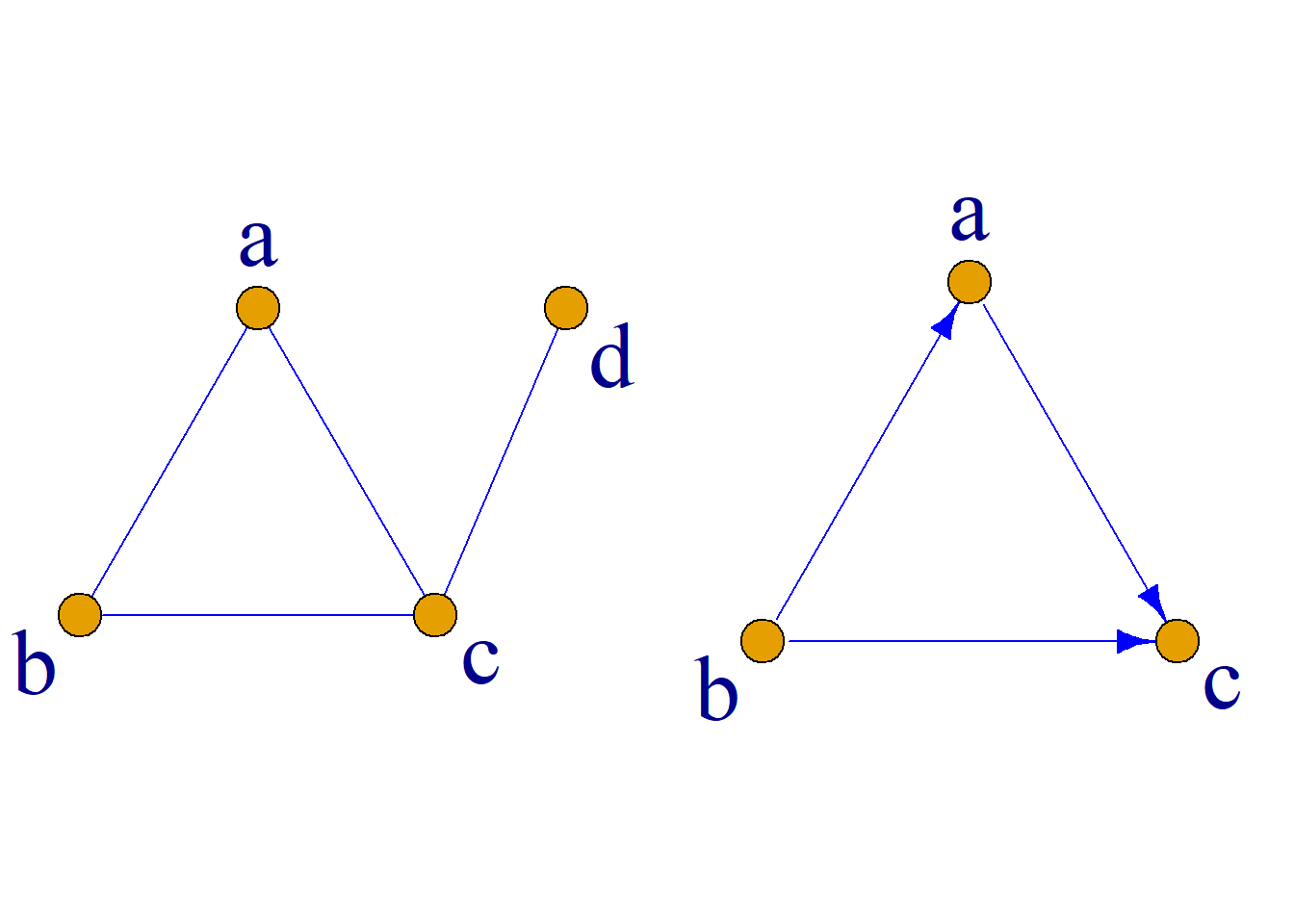
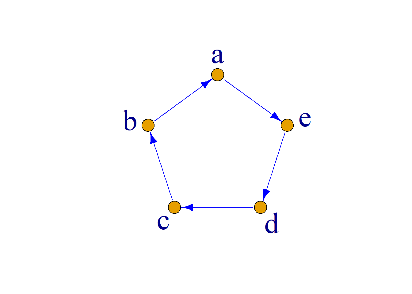
Example: As shown in graph \(G\), \(a\) and \(d\) are mutually reachable, but
\(d[a, d]=2\), \(d[d, a]=3\).
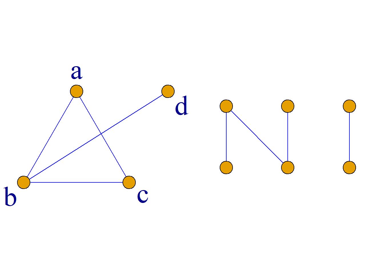
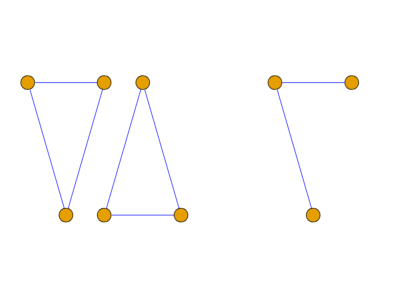
Definition: Given an undirected graph \(G={\langle}V, E{\rangle}\), if every pair of vertices in \(G\) is mutually reachable, then undirected graph \(G\) is called connected; otherwise it is called disconnected.
Undirected graphs are divided into two categories: connected and disconnected.
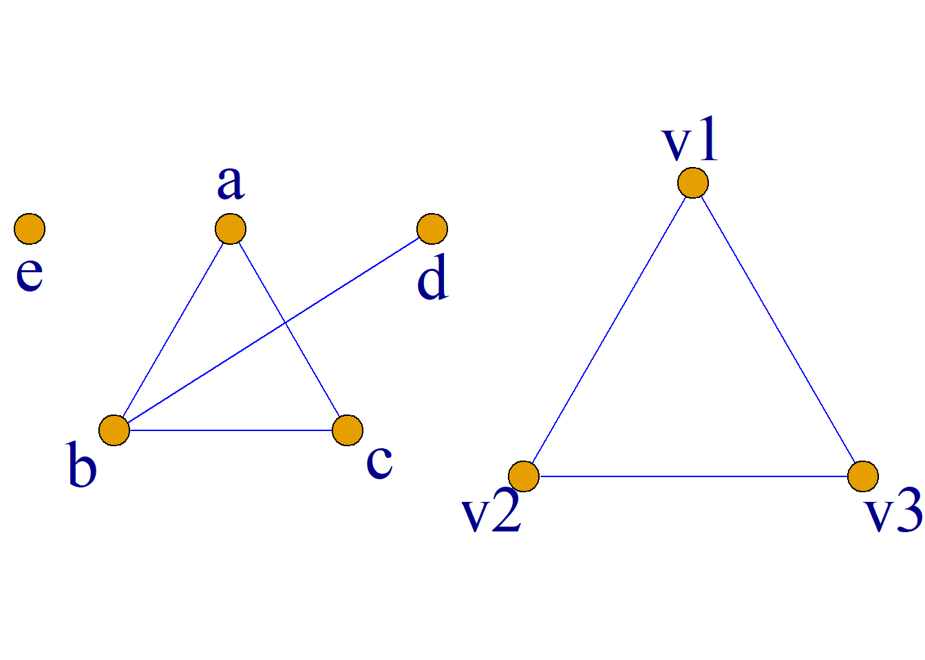
Definition: Let \(G^\prime\) be a subgraph of undirected graph \(G\). If \(G^\prime\) is connected, then \(G^\prime\) is called a connected subgraph of undirected graph \(G\).
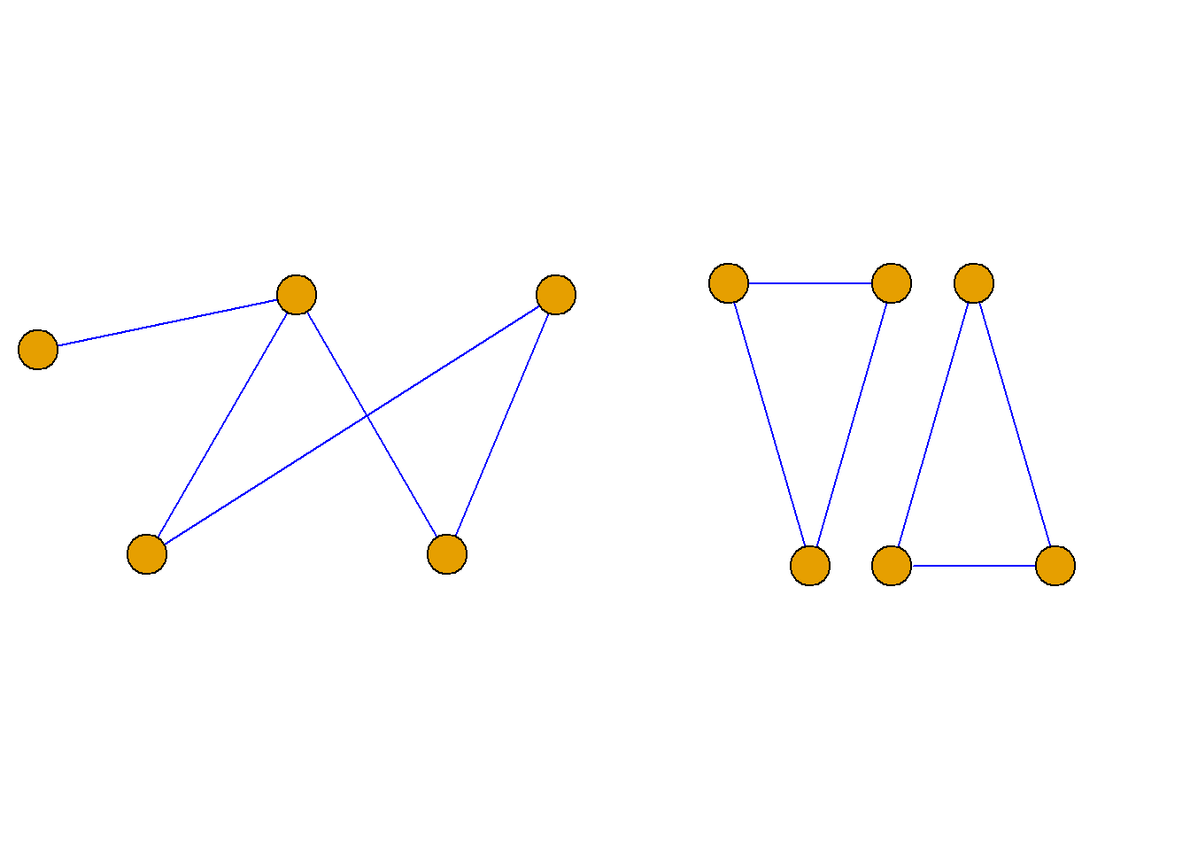
Definition: Let \(G^\prime\) be a connected subgraph of undirected graph \(G\). If \(G^\prime\) is not contained in any larger connected subgraph of \(G\), then \(G^\prime\) is called a connected component (maximal connected subgraph) of undirected graph \(G\).
If an undirected graph \(G\) is connected, then it has only one connected component, namely \(G\) itself; if \(G\) is disconnected, then it has at least two connected components. The number of connected components of an undirected graph is often denoted \(p(G)\) (or \(w(G)\)).
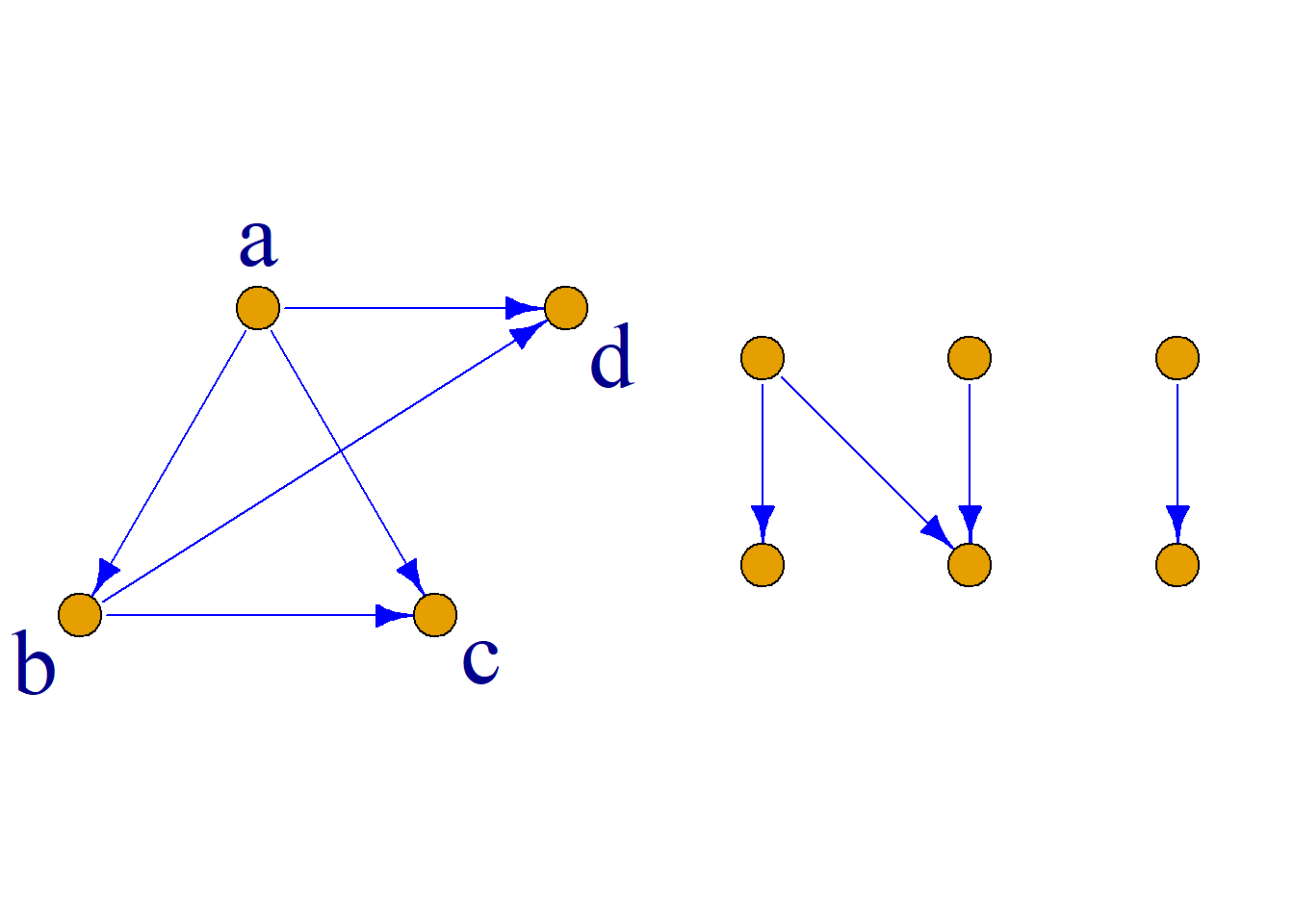
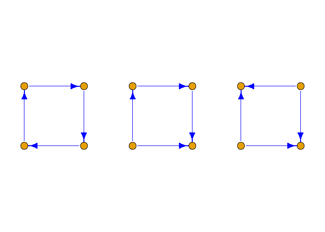
Definition: Let \(G={\langle}V, E{\rangle}\) be a directed graph. Then:
If the undirected graph obtained by ignoring all edge directions in \(G\) is connected, then the directed graph \(G\) is called weakly connected.
If for any two vertices in \(G\), at least one vertex is reachable from the other, then directed graph \(G\) is called unilaterally connected.
If every pair of vertices in \(G\) is mutually reachable, then directed graph \(G\) is called strongly connected.
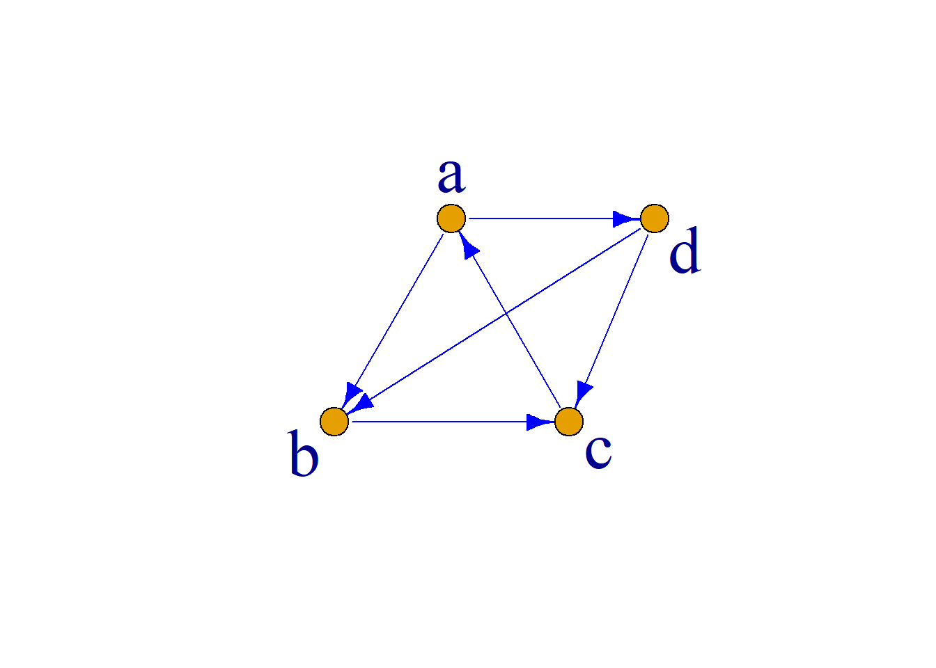
Theorem: A directed graph \(G\) is strongly connected if and only if there exists a circuit in \(G\) that passes through every vertex at least once.
The right graph is a strongly connected graph. A circuit passing through every vertex: bcadb.
Definition: Let \(G^\prime\) be a subgraph of directed graph \(G\) with some property. If no other subgraph of \(G\) has this property and contains \(G^\prime\) as a proper subgraph, then \(G^\prime\) is called a maximal subgraph of \(G\) with that property.
Top left: original graph;
Top right: maximal subgraph with strong connectivity;
Bottom left: maximal subgraph with unilateral connectivity;
Bottom right: maximal subgraph with unilateral connectivity.
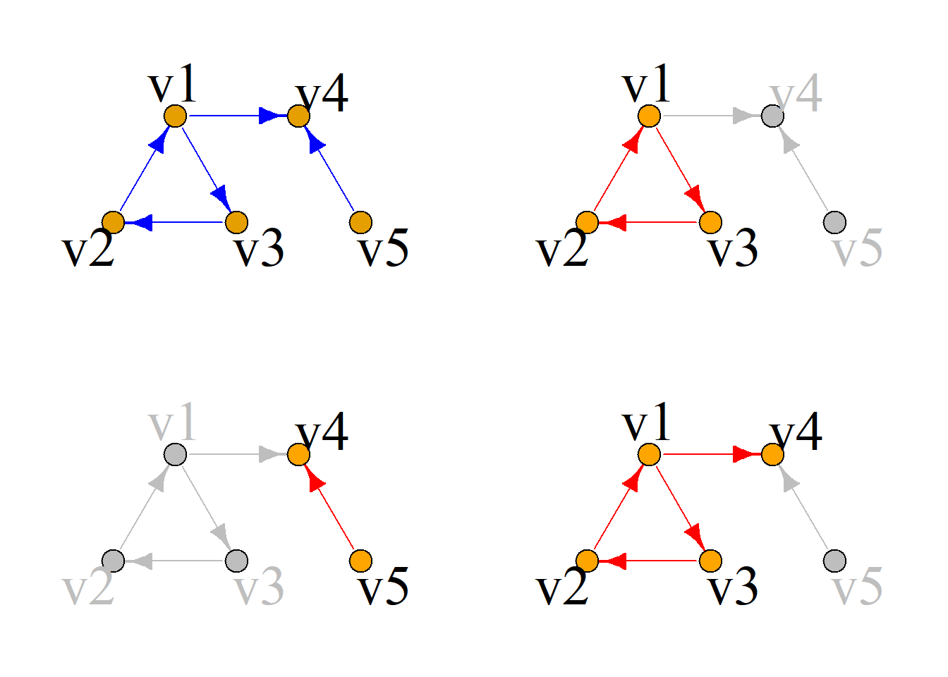
Definition: In a directed graph \(G\), a maximal subgraph with the strongly connected property is called a strong component (strongly connected component); a maximal subgraph with the unilaterally connected property is called a unilateral component (unilaterally connected component); a maximal subgraph with the weakly connected property is called a weak component (weakly connected component).
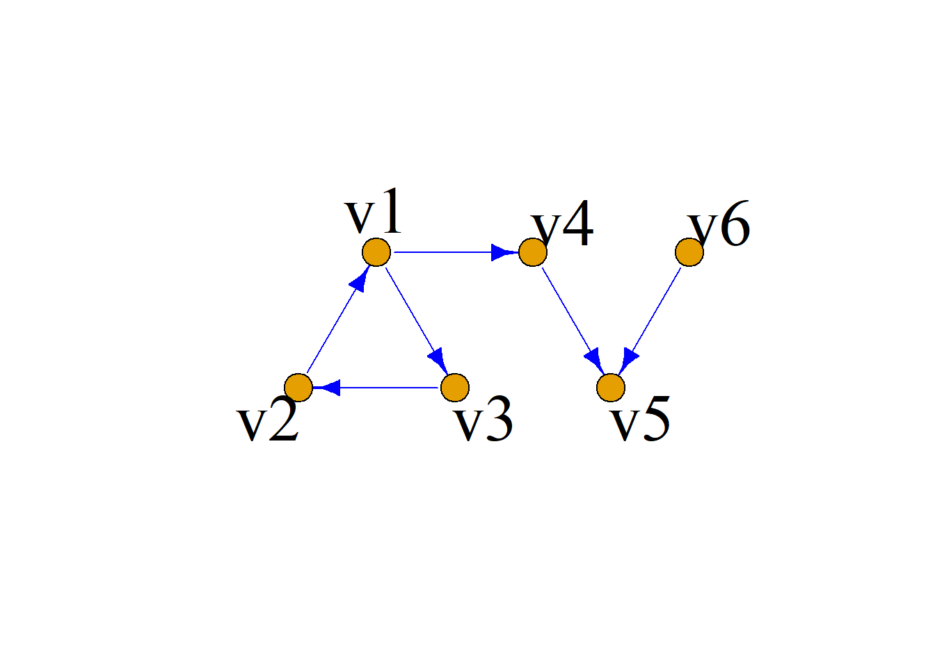
\(G[\{v_1, v_2, v_3\}]\), \(G[\{v_4\}]\), \(G[\{v_5\}]\), \(G[\{v_6\}]\) are strong components;
\(G[\{v_1, v_2, v_3, v_4, v_5\}]\), \(G[\{v_5, v_6\}]\) are unilateral components;
\(G[\{v_1, v_2, v_3, v_4, v_5, v_6\}]\) is a weak component.
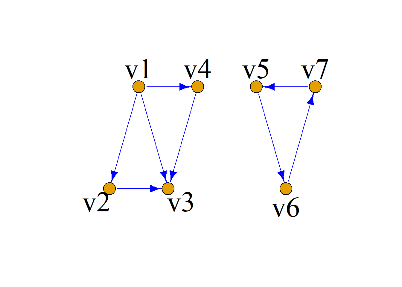
\(G[\{v_1\}]\), \(G[\{v_2\}]\), \(G[\{v_3\}]\), \(G[\{v_4\}]\), \(G[\{v_5, v_6, v_7\}]\) are strong components;
\(G[\{v_1, v_2, v_3\}]\), \(G[\{v_1, v_3, v_4\}]\), \(G[\{v_5, v_6, v_7\}]\) are unilateral components;
\(G[\{v_1, v_2, v_3, v_4\}]\), \(G[\{v_5, v_6, v_7\}]\) are weak components.
Theorem: In a simple directed graph \(G={\langle}V, E{\rangle}\), every vertex belongs to exactly one strong component; every vertex and every edge belongs to exactly one weak component; every vertex and every edge belongs to at least one unilateral component.
Connectivity
Connectivity is a common property of graphs, mainly used to determine the connection status between any two vertices, and is especially useful in detecting network and circuit connections.
Definition: Let undirected graph \(G={\langle}V, E{\rangle}\) be connected. If there exists a vertex subset \(V^\prime{\subset}V\) such that removing \(V^\prime\) from \(G\) yields a disconnected subgraph \(G-V^\prime\), while removing any proper subset of \(V^\prime\) still leaves a connected subgraph, then \(V^\prime\) is called a vertex cut set of \(G\).
If a vertex cut set of graph \(G\) consists of only one vertex \(v\), that vertex \(v\) is called a cut vertex.
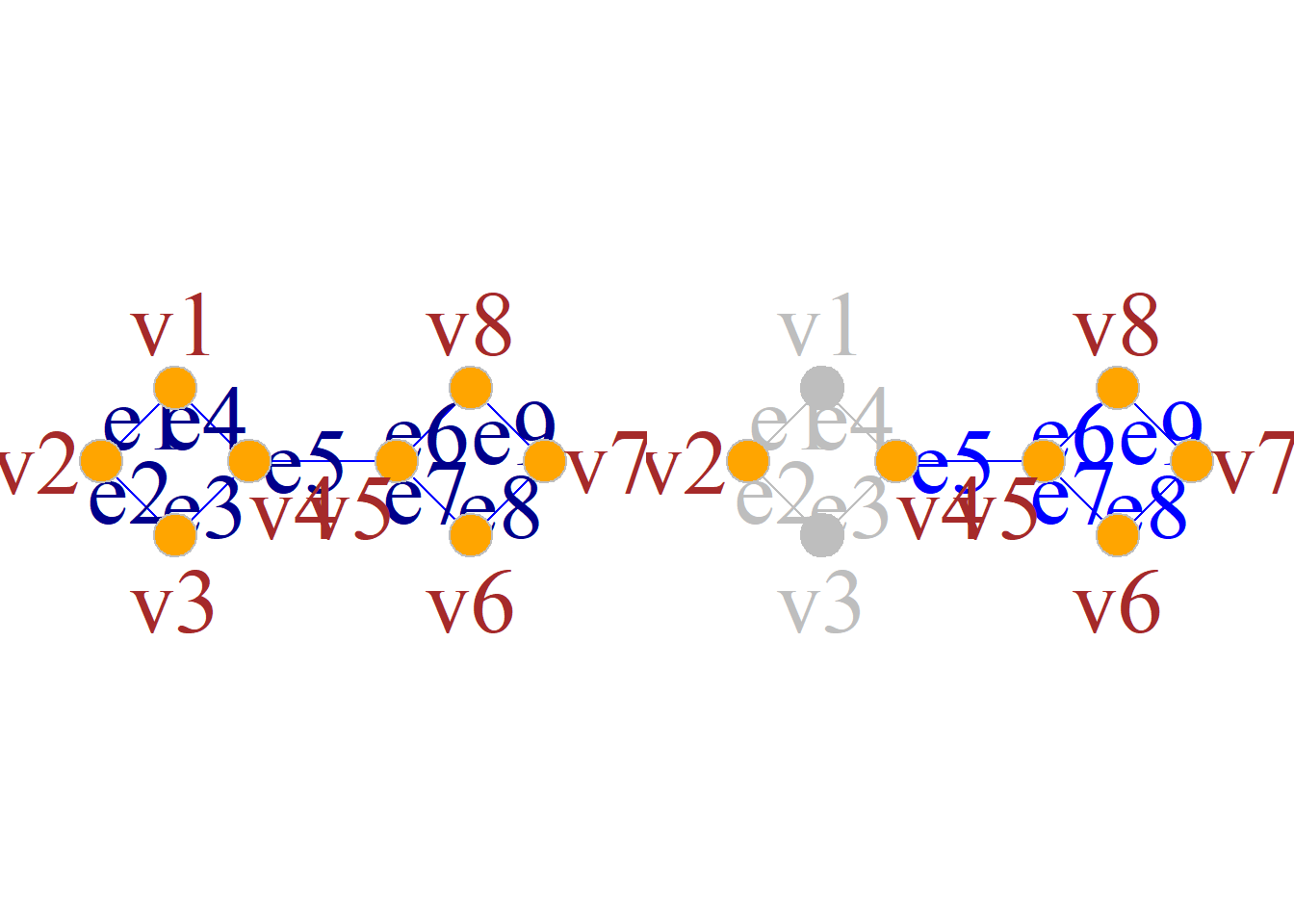
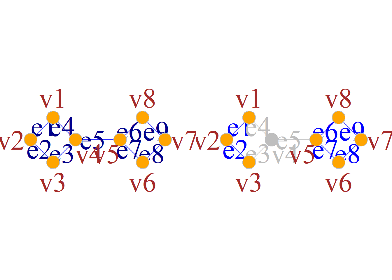
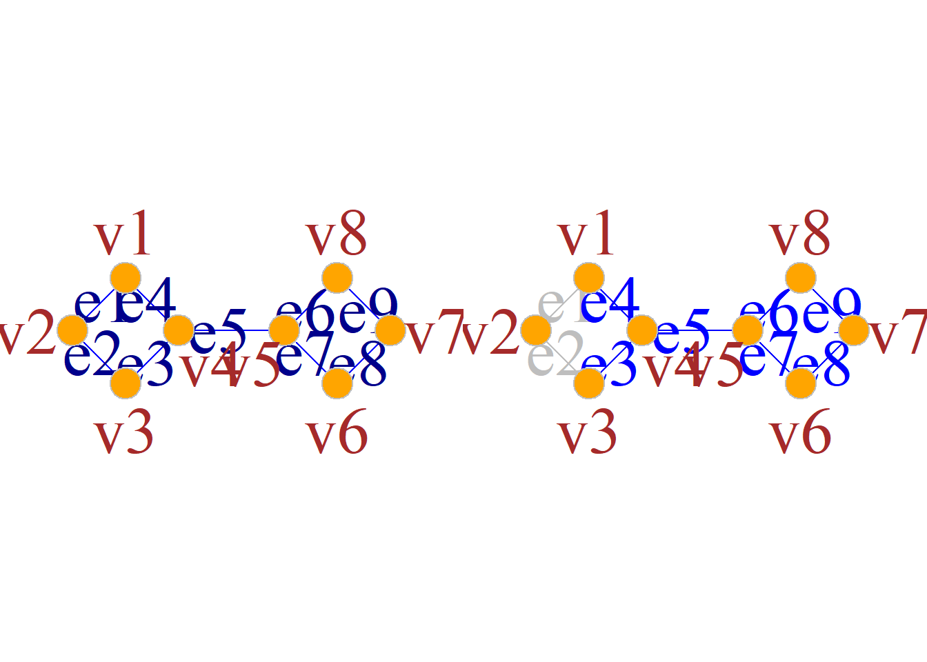
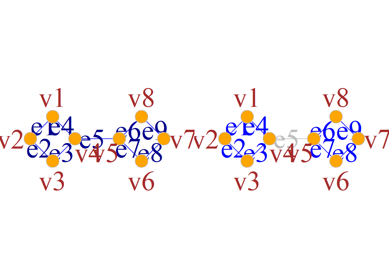
Definition: Let undirected graph \(G={\langle}V, E{\rangle}\) be connected. If there exists an edge subset \(E^\prime{\subset}E\) such that removing \(E^\prime\) from \(G\) yields a disconnected subgraph \(G-E^\prime\), while removing any proper subset of \(E^\prime\) still leaves a connected subgraph, then \(E^\prime\) is called an edge cut set of \(G\).
If an edge cut set of graph \(G\) consists of only one edge \(e\), that edge \(e\) is called a cut edge or bridge.
Definition: Let undirected graph \(G={\langle}V, E{\rangle}\) be connected. Define the vertex connectivity \({\chi}(G)\) of \(G\) as follows:
\({\chi}(G)=\min\{|V^\prime|\, \, |V^\prime\) is a vertex cut set of \(G\) or \(V^\prime\) makes \(G-V^\prime\) a trivial graph}
The vertex connectivity \({\chi}(G)\) is the minimum number of vertices whose deletion from connected graph \(G\) produces a disconnected graph.
If \(G\) is disconnected, then since no vertices need to be deleted for \(G\) to be disconnected, define its vertex connectivity as \[{\chi}(G)=0.\]
Definition: Let undirected graph \(G={\langle}V, E{\rangle}\) be connected. Define the edge connectivity \({\lambda}(G)\) of \(G\) as:
\[ \lambda(G)= \begin{cases} 0 & G\text{ is disconnected}\\ \min\{|E^\prime|\, \, |E^{\prime}\text{ is an edge cut set}\} & \text{otherwise} \end{cases} \]
The edge connectivity \({\lambda}(G)\) is the minimum number of edges whose removal from connected graph \(G\) makes it disconnected.
If \(G\) is disconnected, since \(G\) is already disconnected without removing any edges, we define its edge connectivity \[{\lambda}(G)=0.\]
Example: As shown in the figure,
Vertex connectivity \[{\chi}(G)=1,\] Edge connectivity \[{\lambda}(G)=2.\]
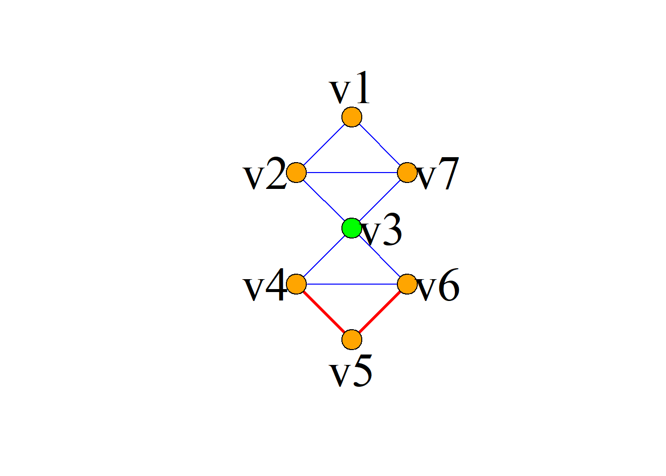
Theorem: For any undirected graph, \[{\chi}(G){\leq}{\lambda}(G){\leq}{\delta}(G)\] Example: As shown in the figure,
Vertex connectivity \[{\chi}(G)=1.\]
Edge connectivity \[{\lambda}(G)=2.\]
Minimum degree \[{\delta}(G)=2.\]
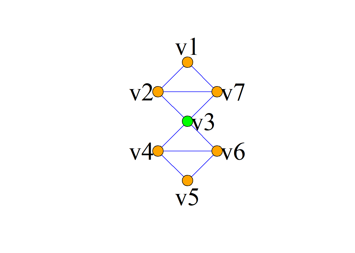
At any gathering of 6 people, there are always 3 people who all know each other, or 3 people who are all strangers to each other. How to prove this?
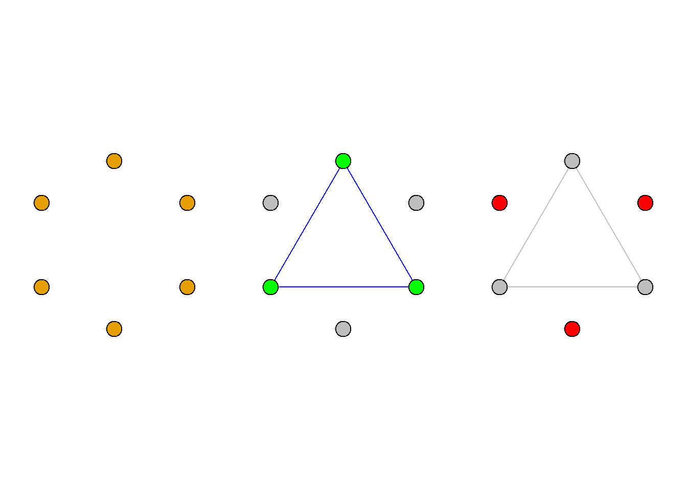
3 people mutually acquainted means \(G\) contains \(K_3\) as a subgraph;
3 people mutually unacquainted means \(G\) contains the \({\langle}3, 0\rangle\) graph as a subgraph.
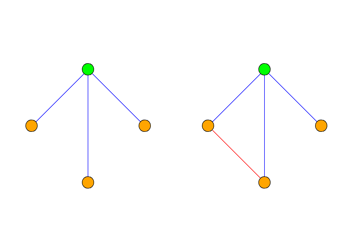
Take any vertex \(v\) in \(V\). There are two cases:
- \(v\) is adjacent to at least 3 other vertices, which further contains two sub-cases:
These three vertices are mutually non-adjacent, so \(G\) contains \({\langle}3, 0{\rangle}\) as a subgraph;
At least two of these three vertices are adjacent, so \(G\) contains \(k_3\) as a subgraph.
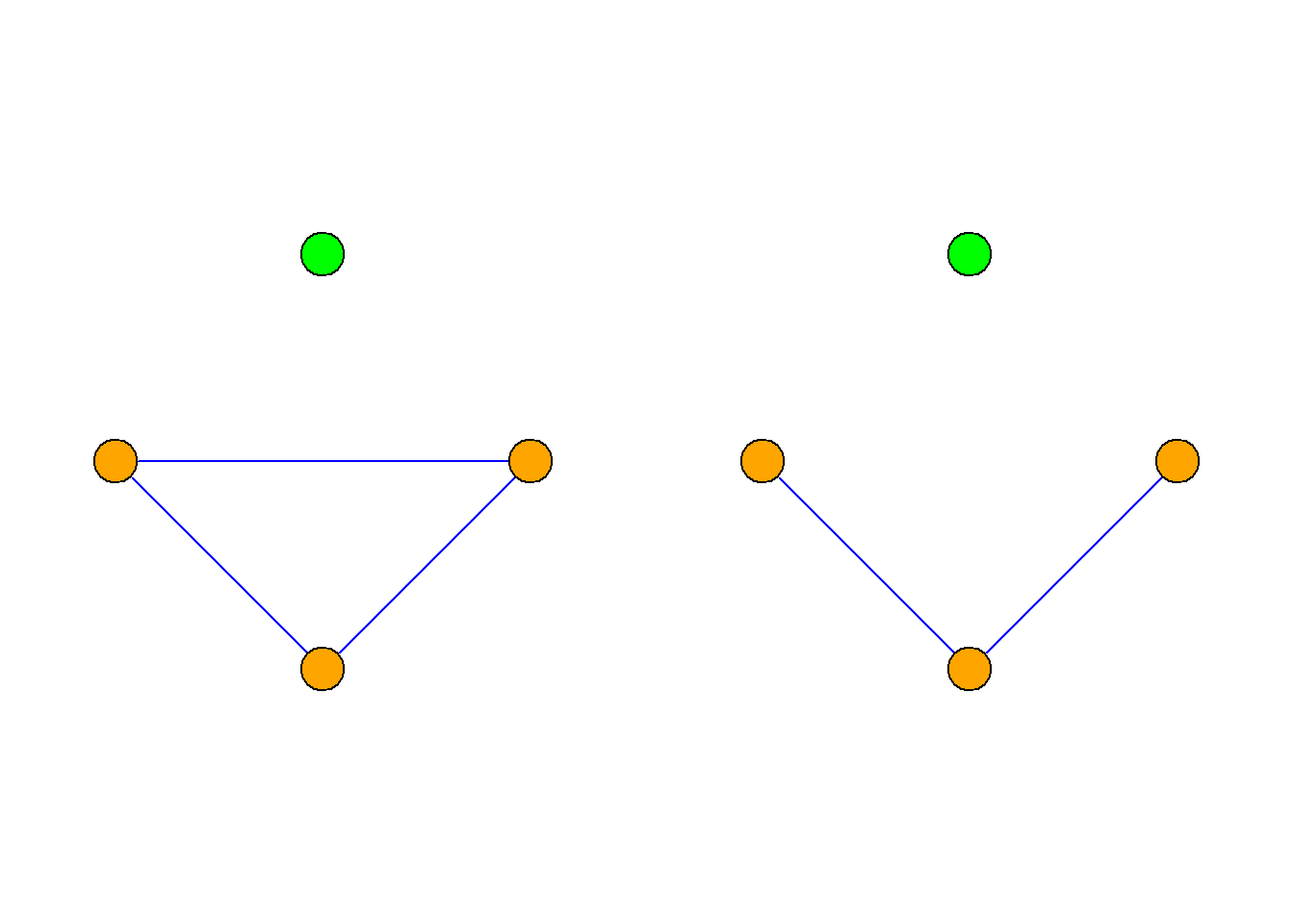
- \(v\) is adjacent to at most 2 other vertices (i.e., non-adjacent to at least 3 others), which further contains two sub-cases:
These 3 vertices are pairwise adjacent, so \(G\) contains \(k_3\) as a subgraph.
At least 2 of these 3 vertices are non-adjacent, so \(G\) contains \({\langle}3, 0{\rangle}\) as a subgraph.
Prove that the number of people who shake hands with an odd number of people at any gathering is even.
Solution: Model the people at the gathering as vertices; connect two vertices if the corresponding people shake hands, forming a simple graph \(G\).
This way, the degree of vertex \(v\) in \(G\) corresponds to the number of people who shook hands with \(v\). Thus, the problem reduces to proving that the number of odd-degree vertices in \(G\) is even.
By the theorem “in any graph \(G={\langle}V, E{\rangle}\), the number of vertices with odd degree must be even”, the result follows.
The mathematical abstraction of a graph is a triple; its intuitive visual representation is a graph diagram.
For ease of computation, graphs can also be represented by matrices. The relationships between vertices, between vertices and edges, and between edges and circuits can all be expressed by matrices.
We can fully exploit the operations of matrix algebra to study the structural properties of graphs, which facilitates computer processing of graphs.
Matrix Representation of Graphs
General Graphs
Incidence Matrix Definition: Let \(G={\langle}V, E{\rangle}\) be an undirected graph, \(V=\{v_1, v_2, {\cdots}, v_n\}\), \(E=\{e_1, e_2, {\cdots}, e_m\}\). Let \(m_{ij}\) be the number of times vertex \(v_i\) is incident with edge \(e_j\). The matrix \((m_{ij})_{n{\times}m}\) is called the incidence matrix of \(G\), denoted \(M(G)\) or \(M\).
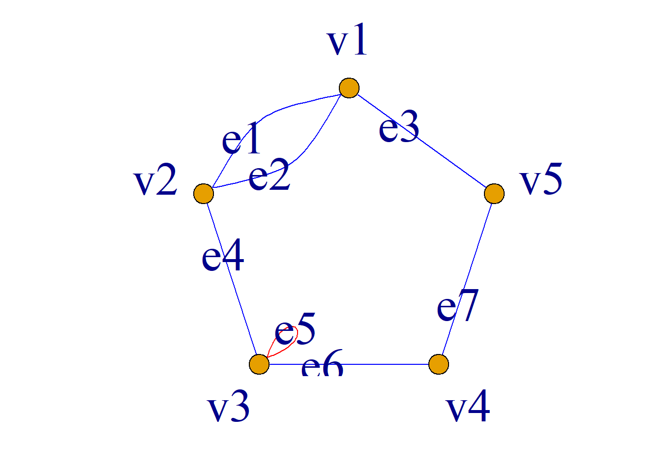
Example: The undirected graph \(G\) is shown as; its incidence matrix \(M\) is:
\[ \left( \begin{aligned} 1&1&1&0&0&0&0\\ 1&1&0&1&0&0&0\\ 0&0&0&1&2&1&0\\ 0&0&0&0&0&1&1\\ 0&0&1&0&0&0&1\\ \end{aligned} \right) \]
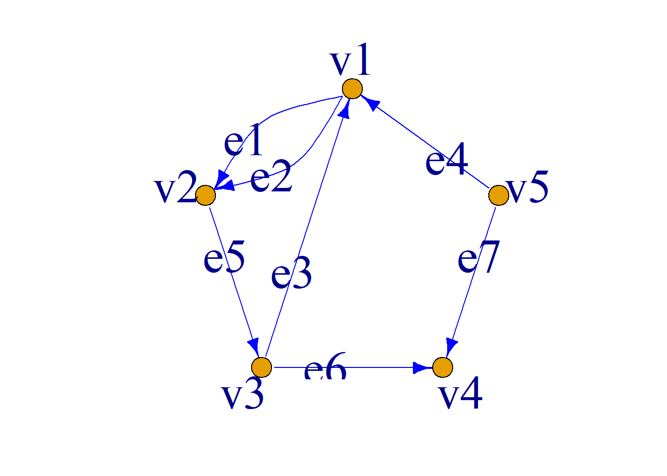
Definition: Let \(G={\langle}V, E{\rangle}\) be a directed acyclic graph, \(V=\{v_1, v_2, {\cdots}, v_n\}\), \(E=\{e_1, e_2, {\cdots}, e_m\}\). Then the matrix \(M(G)=(m_{ij})_{n{\times}m}\) is called the incidence matrix of \(G\), abbreviated as \(M\). where: \[ m_{ij}= \begin{cases} 0 & \text{if } e_j \text{ is not incident with } v_i \\ 1 & \text{if } v_i \text{ is the initial vertex of } e_j \\ -1 & \text{if } v_i \text{ is the terminal vertex of } e_j \\ \end{cases} \] Example: The directed graph \(G\) is shown; its incidence matrix \(M\) is: \[\left( \begin{aligned} 1&1&-1&-1&0&0&0\\ -1&-1&0&0&1&0&0\\ 0&0&1&0&-1&1&0\\ 0&0&0&0&0&-1&-1\\ 0&0&0&1&0&0&1\\ \end{aligned} \right) \]
Definition: Let \(G={\langle}V, E{\rangle}\) be an undirected graph, \(V=\{v_1, v_2, {\cdots}, v_n\}\), then the \(n{\times}n\) matrix \(A(G)=(a_{ij})_{n{\times}n}\) is called the adjacency matrix of \(G\). Abbreviated as \(A\). where: \(a_{ij}\) is the number of edges with both \(v_i\) and \(v_j\) as endpoints.
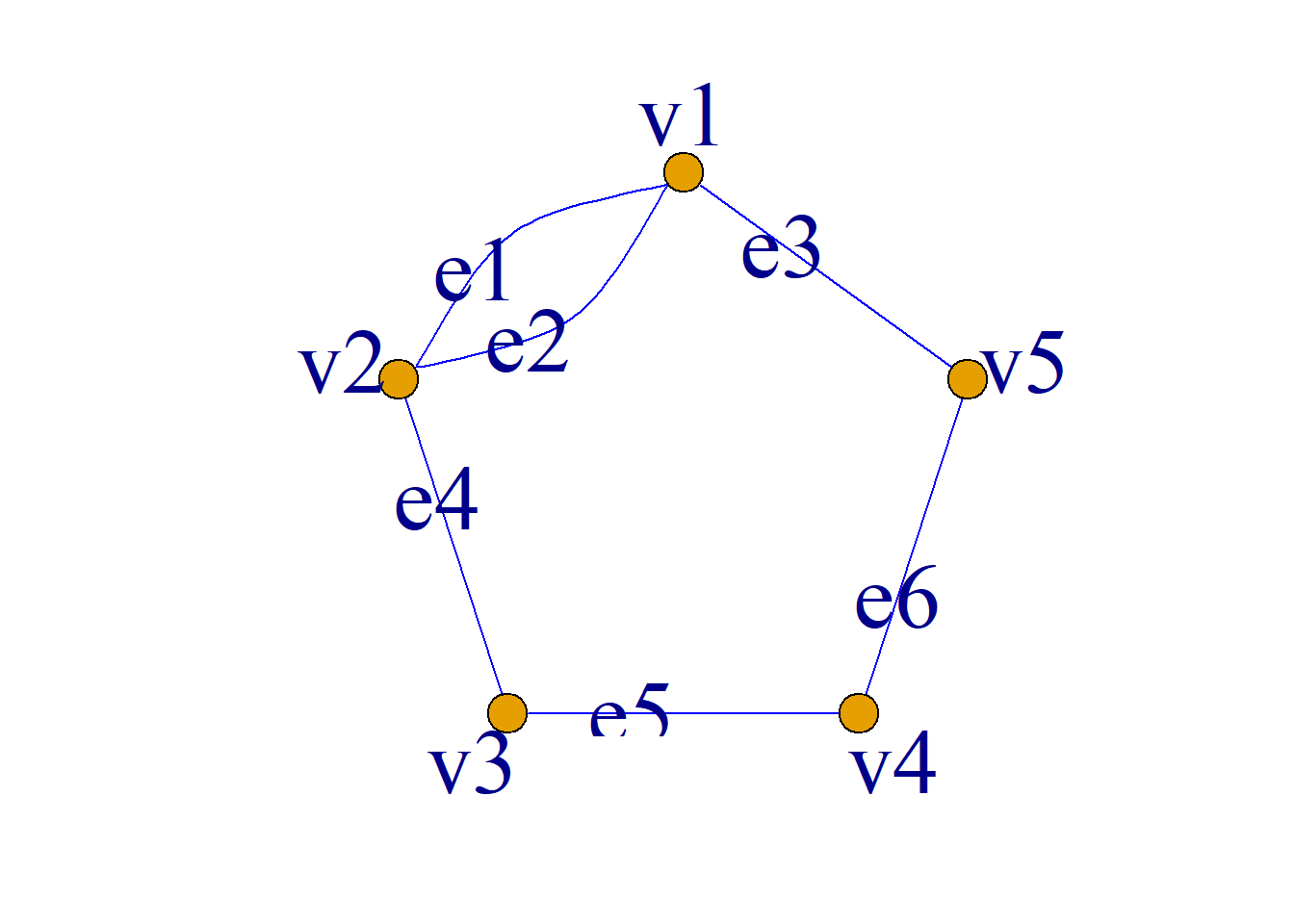
Example: The undirected graph \(G\) is shown; its adjacency matrix \(M\) is:
\[\left( \begin{aligned} 0&2&0&0&1\\ 2&0&1&0&0\\ 0&1&0&1&0\\ 0&0&1&0&1\\ 1&0&0&1&0\\ \end{aligned} \right) \] ’
Definition: Let \(G={\langle}V, E{\rangle}\) be a directed graph, \(V=\{v_1, v_2, {\cdots}, v_n\}\), then the \(n{\times}n\) matrix
\(A(G)=(a_{ij})_{n{\times}n}\)
is called the adjacency matrix of \(G\). Abbreviated as \(A\). where: \(a_{ij}\) is the number of edges directed from \(v_i\) to \(v_j\).
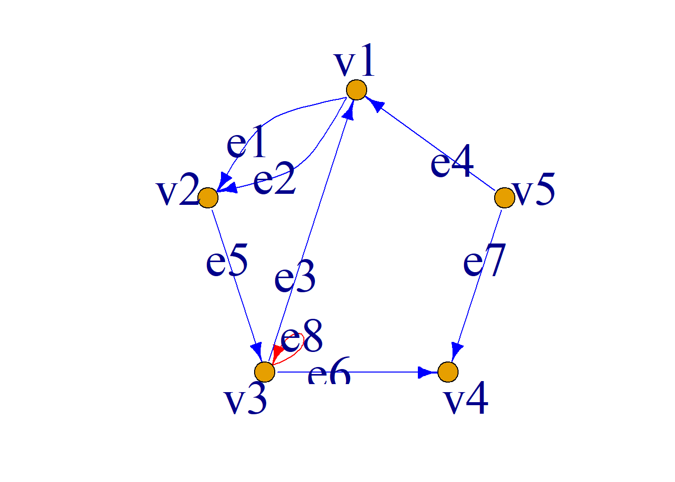
Example: The directed graph \(G\) is shown; its adjacency matrix \(A\) is:
\[\left( \begin{aligned} 0&2&0&0&1\\ 0&0&1&0&0\\ 1&0&1&1&0\\ 0&0&0&0&0\\ 1&0&0&1&0\\ \end{aligned} \right) \]
Simple Graphs
Definition: Let \(G={\langle}V, E{\rangle}\) be a simple undirected graph, \(V=\{v_1, v_2, {\cdots}, v_n\},\,E=\{e_1, e_2, {\cdots}, e_m\}\), The matrix \(M=(m_{ij})_{n{\times}m}\) is called the incidence matrix of \(G\), where:
\[ m_{ij}= \begin{cases} 1 & \text{if } e_j \text{ is incident with } v_i \\ 0 & \text{if } e_j \text{ is not incident with } v_i \\ \end{cases} \]
The incidence matrix \(M\) of a simple undirected graph has the following properties:
Each column of the matrix has exactly two 1s, since each edge is incident with two vertices.
The sum of elements in each row equals the degree of the corresponding vertex.
If all elements in a row are 0, the corresponding vertex is an isolated vertex.
Example: The simple undirected graph \(G\) is shown; its incidence matrix \(M\) is: \[\left( \begin{aligned} 1&0&1&0&1&0&1\\ 1&1&0&0&0&0&0\\ 0&1&1&1&0&0&0\\ 0&0&0&1&1&1&0\\ 0&0&0&0&0&1&1\\ \end{aligned} \right) \]
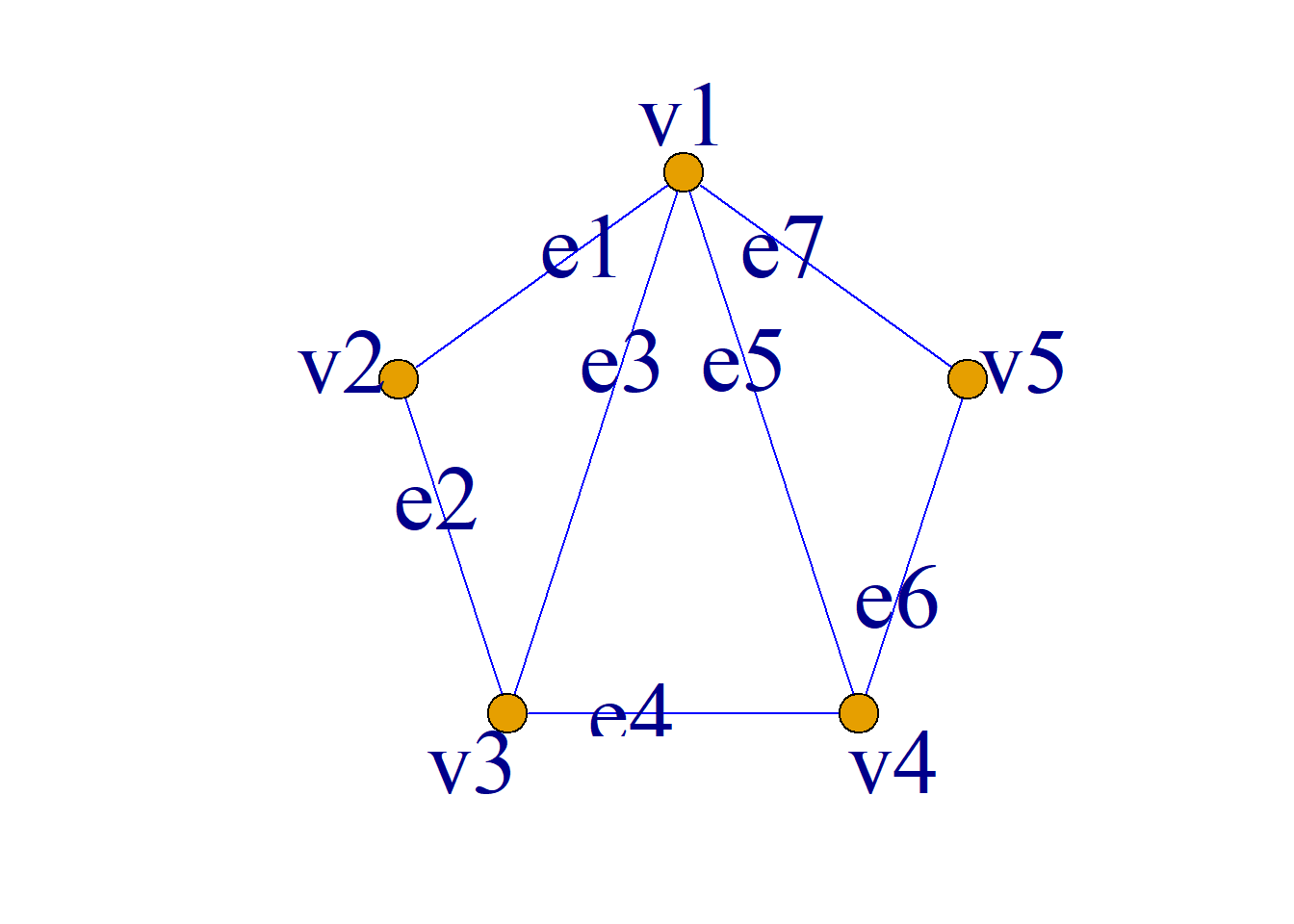
Definition: Let \(G={\langle}V, E{\rangle}\) be a simple directed graph, \(V=\{v_1, v_2, {\cdots}, v_n\}\), \(E=\{e_1, e_2, {\cdots}, e_m\}\). Then the matrix \(M=(m_{ij})_{n{\times}m}\) is called the incidence matrix of \(G\), where: \[ m_{ij}= \begin{cases} 0 & \text{if } e_j \text{ is not incident with } v_i \\ 1 & \text{if } v_i \text{ is the initial vertex of } e_j \\ -1 & \text{if } v_i \text{ is the terminal vertex of } e_j \\ \end{cases} \]
The incidence matrix \(M\) of a simple directed graph has the following properties:
The sum of elements in each column is 0, since each edge is incident with two vertices: one initial vertex and one terminal vertex.
The sum of absolute values of elements in each row equals the degree of the corresponding vertex.
The algebraic sum of all elements in the matrix is 0.
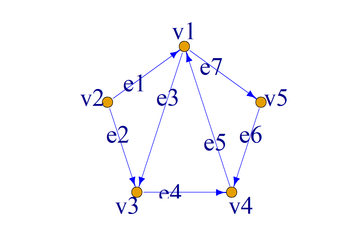
Example: The simple directed graph \(G\) is shown; its incidence matrix \(M\) is:
\[\left( \begin{aligned} -1&0&1&0&-1&0&1\\ 1&1&0&0&0&0&0\\ 0&-1&-1&1&0&0&0\\ 0&0&0&-1&1&-1&0\\ 0&0&0&0&0&1&-1\\ \end{aligned} \right) \]
Definition: Let \(G={\langle}V, E{\rangle}\) be a simple undirected graph, \(V=\{v_1, v_2, {\cdots}, v_n\}\) then the \(n{\times}n\) matrix \(A=(a_{ij})_{n{\times}n}\) is called the adjacency matrix of \(G\), where:
\[ a_{ij}= \begin{cases} 1 & \text{if } (v_i, v_j){\in}E \\ 0 & \text{if } (v_i, v_j){\notin}E \\ \end{cases} \] Example: The adjacency matrix of simple undirected graph \(G\) is: \[\left( \begin{aligned} 0&1&1&0&1\\ 1&0&0&0&0\\ 1&0&0&0&1\\ 0&0&0&0&1\\ 1&0&1&1&0\\ \end{aligned} \right) \]
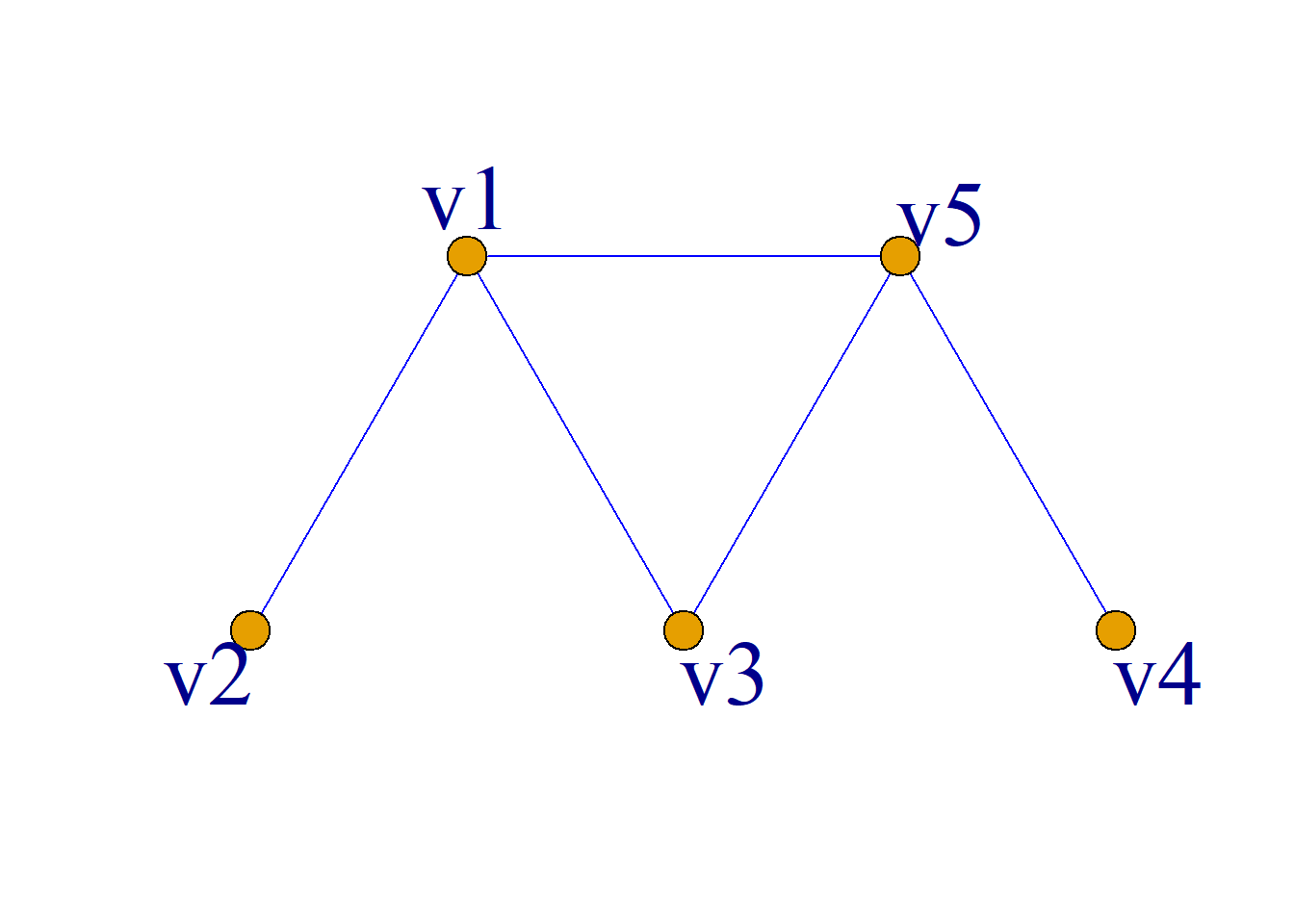
Definition: Let \(G={\langle}V, E{\rangle}\) be a simple directed graph, \(V=\{v_1, v_2, {\cdots}, v_n\}\), then the \(n{\times}n\) matrix \(A=(a_{ij})_{n{\times}n}\) is called the adjacency matrix of \(G\), where:
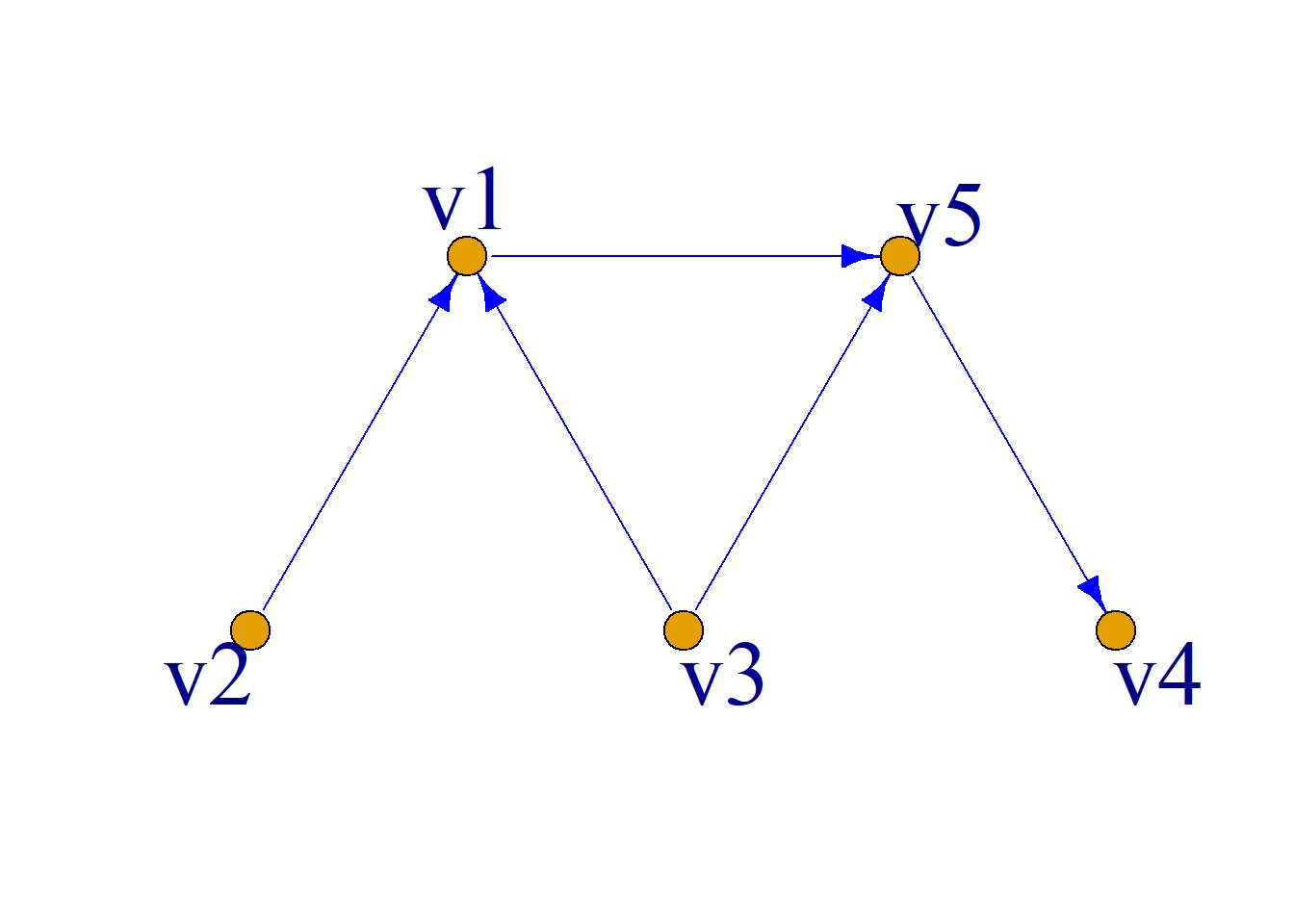
\[ a_{ij}= \begin{cases} 1 & \text{if } {\langle}v_i, v_j{\rangle}{\in}E \\ 0 & \text{if } {\langle}v_i, v_j{\rangle}{\notin}E \\ \end{cases} \] Example: The adjacency matrix of simple directed graph \(G\) is:
\[\left( \begin{aligned} 0&0&0&0&1\\ 1&0&0&0&0\\ 1&0&0&0&1\\ 0&0&0&0&0\\ 0&0&0&1&0\\ \end{aligned} \right) \]
The adjacency matrix of a simple undirected graph is symmetric; that of a simple directed graph is not necessarily symmetric.
By the definition of adjacency matrix, the adjacency matrix of a graph depends on the labeling order of vertices; different orderings produce different adjacency matrices.
However, adjacency matrices from two different vertex orderings are closely related: one can be obtained from the other by simply swapping certain rows and the corresponding columns.
The adjacency matrices of \(G_1\) and \(G_2\) respectively are:
\[\left( \begin{aligned} 0&0&0&1\\ 1&0&0&0\\ 1&0&0&1\\ 0&0&0&0\\ \end{aligned} \right) \] \[ \left( \begin{aligned} 0&1&0&0\\ 0&0&0&1\\ 0&1&0&1\\ 0&0&0&0\\ \end{aligned} \right) \] Swap rows 1, 2 and columns 1, 2.
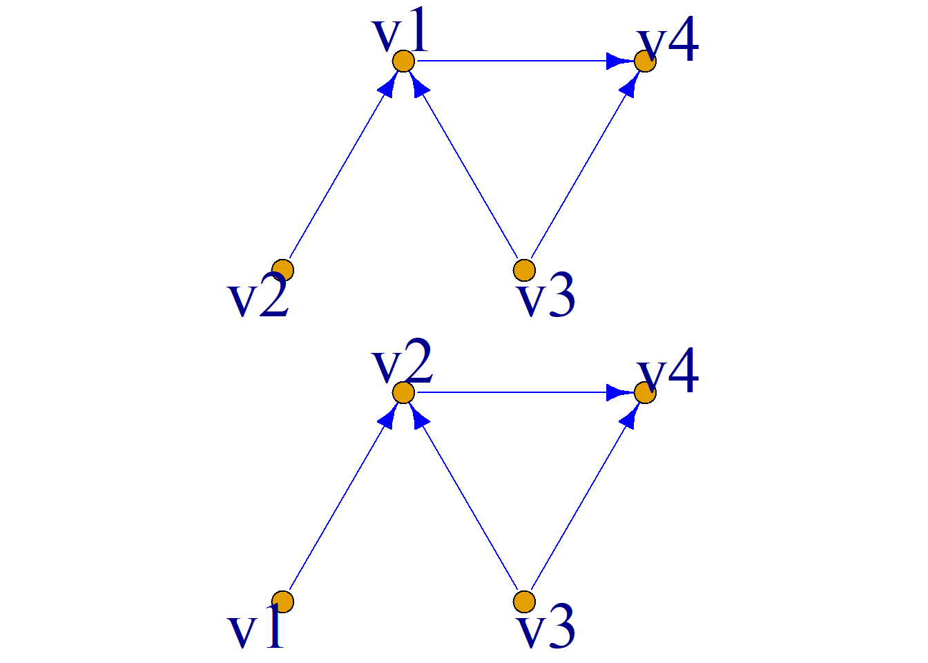
Since \(n\) vertices have \(n!\) different orderings, a graph with \(n\) vertices has \(n!\) different adjacency matrices.
In general, the ordering of vertices in \(G\) is fixed to make its adjacency matrix unique.
Every simple graph corresponds to such a Boolean matrix. Conversely, a Boolean matrix with all zeros on the main diagonal uniquely defines a simple graph.
\[ \left( \begin{aligned} 0&1&1&1\\ 1&0&0&0\\ 1&0&0&1\\ 1&0&1&0\\ \end{aligned} \right) \]
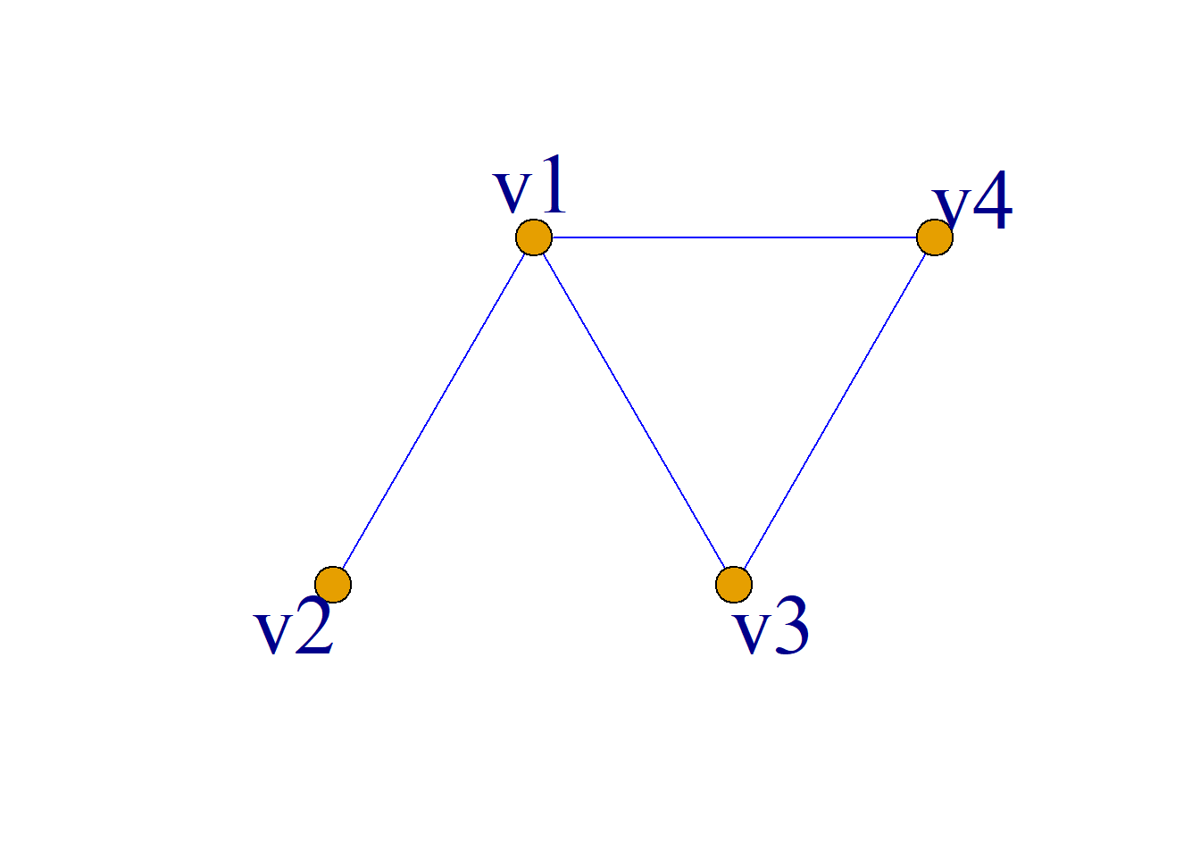
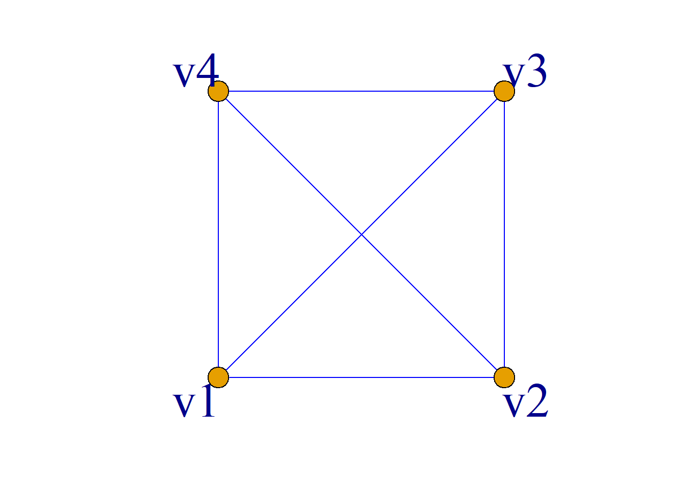
The adjacency matrix reflects some basic properties of a simple graph: if all entries except the main diagonal are 1, then the corresponding graph is a complete graph.
\[ \left( \begin{aligned} 0&1&1&1\\ 1&0&1&1\\ 1&1&0&1\\ 1&1&1&0\\ \end{aligned} \right) \]
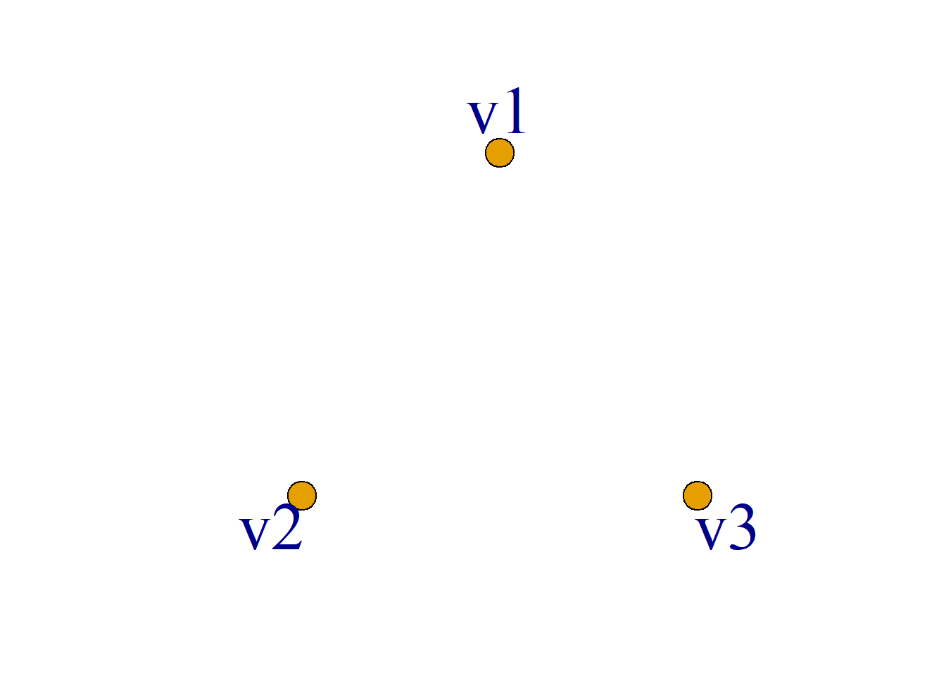
If an adjacency matrix is a zero matrix, then the corresponding graph is a null graph.
\[ \left( \begin{aligned} 0&0&0\\ 0&0&0\\ 0&0&0\\ \end{aligned} \right) \]
Moreover, some quantitative properties of the corresponding graph can be obtained by performing certain operations on the adjacency matrix.
Let the adjacency matrix of simple directed graph \(G={\langle}V, E{\rangle}\) be \(A=(a_{ij})_{n{\times}n}\), \(A^T\) be the transpose of \(A\), define \(B=(b_{ij})_{n{\times}n}\), \(C=(c_{ij})_{n{\times}n}\), where \(B=A{\times}A^T\), \(C=A^T{\times}A\). \({\times}\) denotes matrix multiplication.
In matrix \(A\), the number of 1s in row \(i\) equals the out-degree of vertex \(v_i\); the number of 1s in column \(i\) equals the in-degree of vertex \(v_i\); the sum of the number of 1s in row \(i\) and the number of 1s in column \(i\) equals the degree of vertex \(v_i\).
That is: \[d^+(v_i)=\sum_{k=1}^na_{ik}, \,\,d^-(v_i)=\sum_{k=1}^na_{ki}, \,\,d(v_i)=\sum_{k=1}^n(a_{ki}+a_{ik}).\]
For matrix \(B=A{\times}A^T\), the element \(b_{ij}\) in row \(i\) and column \(j\):
\[b_{ij}=\sum_{k=1}^na_{ik}a_{jk}\]
represents the number of common terminal vertices among edges departing from \(v_i\) and \(v_j\) respectively.
In particular, the diagonal element \(b_{ii}\) is the out-degree of vertex \(v_i\).
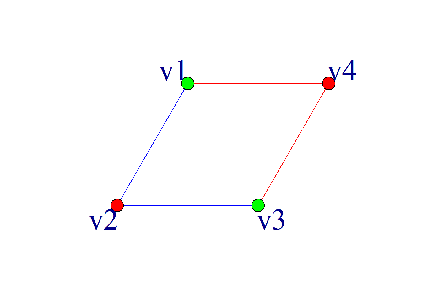
For matrix \(C=A^T{\times}A\), the element \(c_{ij}\) in row \(i\) and column \(j\): \[c_{ij}=\sum_{k=1}^na_{ki}a_{kj}\] represents the number of common initial vertices among edges terminating at \(v_i\) and \(v_j\). In particular, the diagonal element \(c_{ii}\) is the in-degree of vertex \(v_i\).
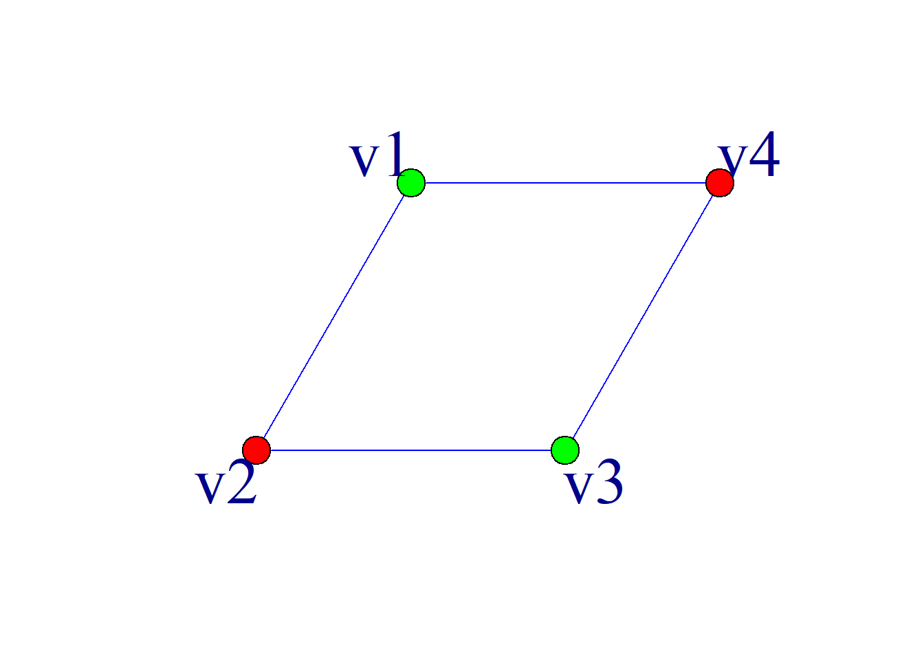
Example:
\[A= \left( \begin{aligned} 0&0&0&1\\ 1&0&0&0\\ 1&1&0&1\\ 1&1&1&0\\ \end{aligned} \right) \]
In matrix \(A\), the number of 1s in row 4 is 3, which equals the out-degree of vertex \(v_4\) in the graph; the number of 1s in column 2 is 2, which equals the in-degree of vertex \(v_2\); the sum of 1s in row 3 and column 3 is 4, which equals the degree of vertex \(v_3\).
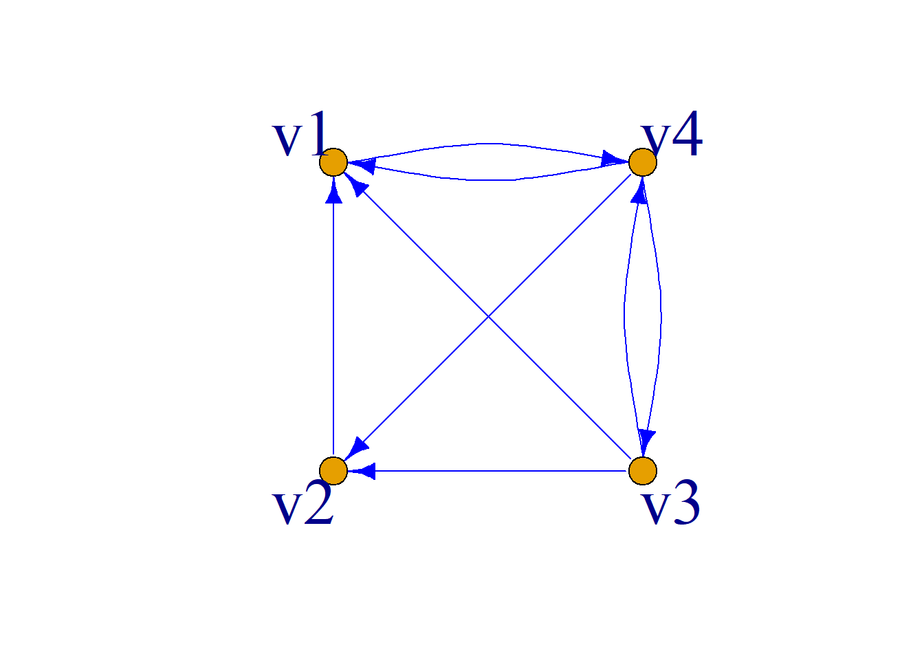
Also: \(B=A{\times}A^T=\)
\[ \left( \begin{aligned} 0&0&0&1\\ 1&0&0&0\\ 1&1&0&1\\ 1&1&1&0\\ \end{aligned} \right) \left( \begin{aligned} 0&1&1&1\\ 0&0&1&1\\ 0&0&0&1\\ 1&0&1&0\\ \end{aligned} \right) \] \[ B=\left( \begin{aligned} 1&0&1&0\\ 0&1&1&1\\ 1&1&3&2\\ 0&1&2&3\\ \end{aligned} \right) \]
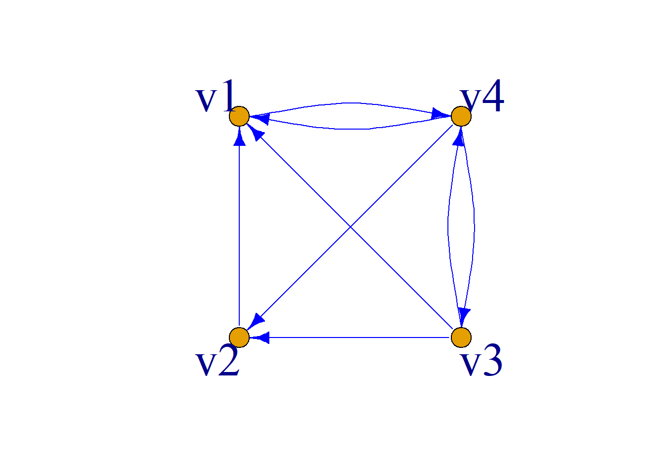
Furthermore:
\(C=A^T{\times}A=\)
\[ \left( \begin{aligned} 0&1&1&1\\ 0&0&1&1\\ 0&0&0&1\\ 1&0&1&1\\ \end{aligned} \right) \left( \begin{aligned} 0&0&0&1\\ 1&0&0&0\\ 1&1&0&1\\ 1&1&1&0\\ \end{aligned} \right) \] \[ C=\left( \begin{aligned} 3&2&1&1\\ 2&2&1&1\\ 1&1&1&0\\ 1&1&0&2\\ \end{aligned} \right) \]
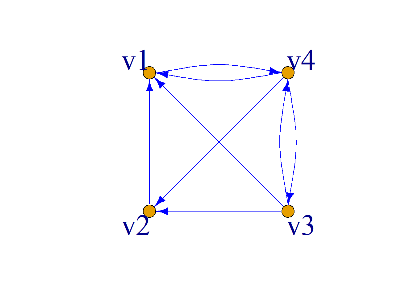
Theorem: Let \(A=(a_{ij})_{n{\times}n}\) be the adjacency matrix of a simple directed graph \(G={\langle}V, E{\rangle}\), and let \(A^l=(a_{ij}^{(l)})_{n{\times}n}\) be the product of \(l\) copies of \(A\). Then:
The element \(a_{ij}^{(l)}\) in row \(i\) and column \(j\) of \(A^l\) is exactly the number of walks of length \(l\) from \(v_i\) to \(v_j\). In particular, the diagonal element \(a_{ii}^{(l)}\) is the number of closed walks of length \(l\) at \(v_i\);
The sum of all elements of \(A^l\) is exactly the number of walks of length \(l\) in \(G\);
\(B_r=(b_{ij}^{(r)})_{n{\times}n}=A+A^2+{\cdots}+A^r\) where \(b_{ij}^{(r)}\) is exactly the number of walks of length at most \(r\) from \(v_i\) to \(v_j\);
The sum of all elements of \(B_r\) is the number of walks of length at most \(r\) in \(G\).
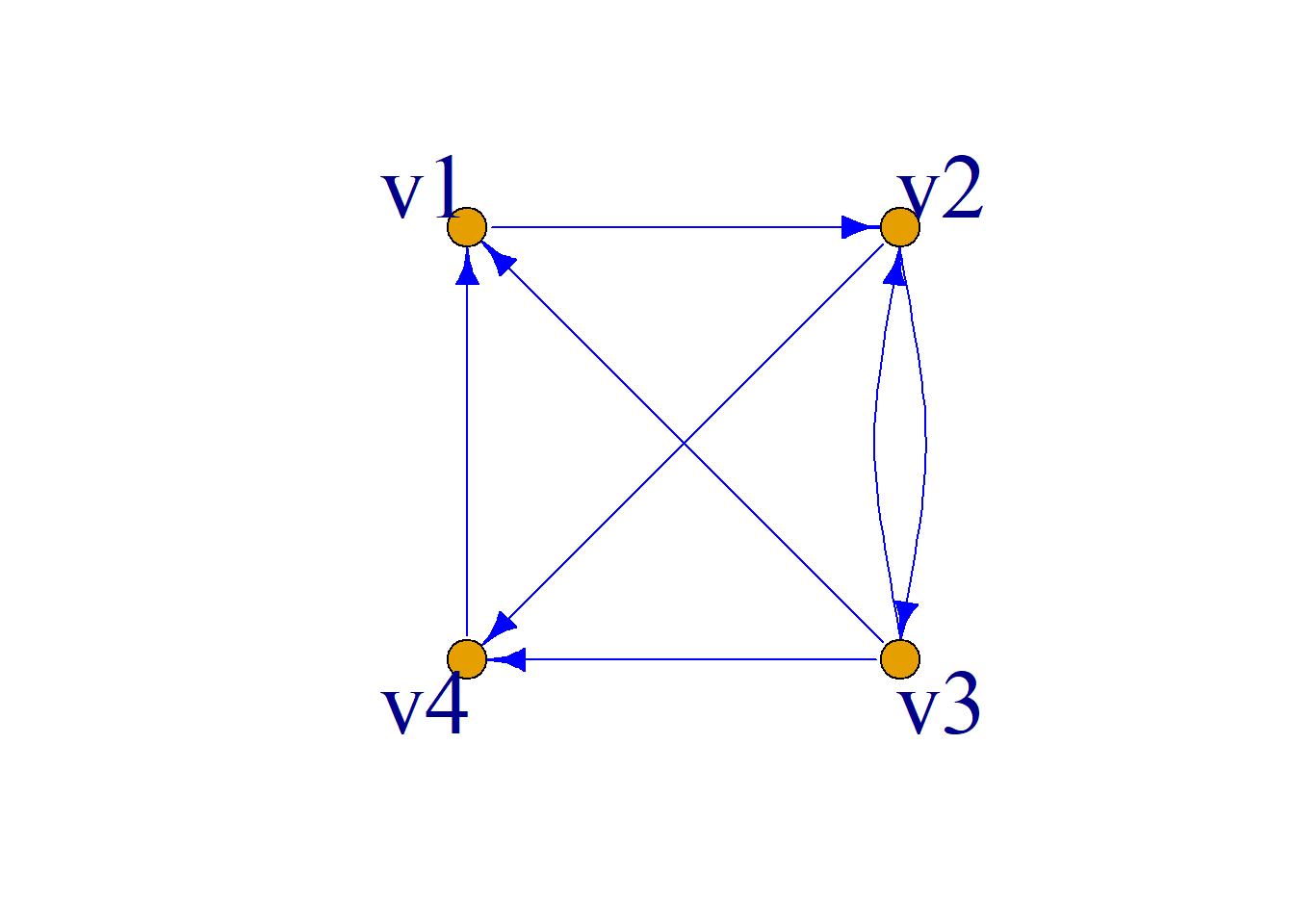
Example: Given simple directed graph \(G\) shown in the figure, its adjacency matrix is \[ \left( \begin{aligned} 0&1&0&0\\ 0&0&1&1\\ 1&1&0&1\\ 1&0&0&0\\ \end{aligned} \right) \]
\[\sum_{i=1}^4\sum_{j=1}^4a_{ij}=7, \sum_{i=1}^4a_{ii}=0\] In the graph, \(a_{23}=1\) indicates there is 1 walk of length 1 from \(v_2\) to \(v_3\); \(a_{42}=0\) indicates there is no walk of length 1 from \(v_4\) to \(v_2\); The sum of elements in \(A\) is 7, indicating there are 7 walks of length 1 in \(G\); The diagonal elements of \(A\) are all 0, indicating there are no cycles of length 1 in \(G\).
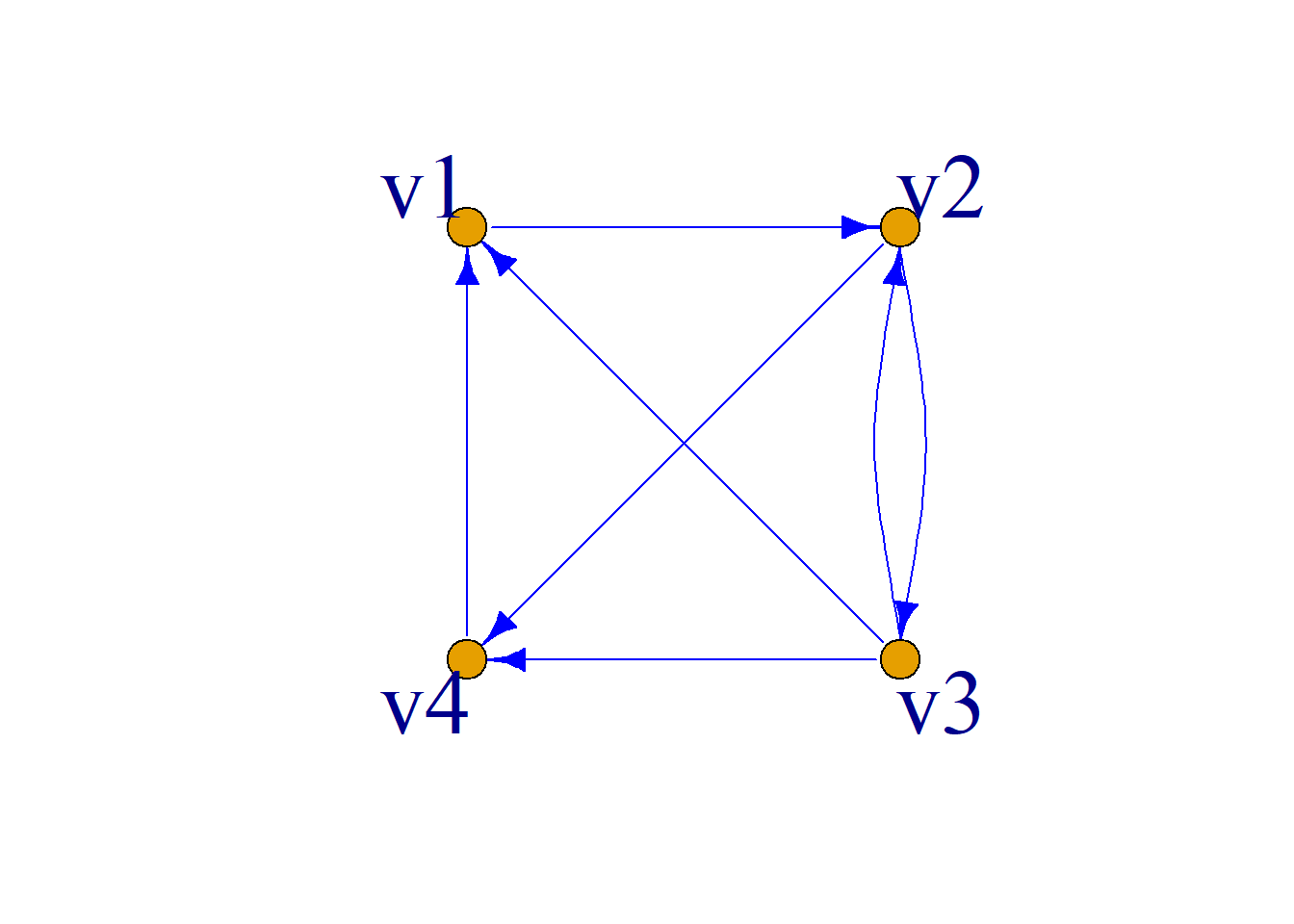
\[ A^2=\left( \begin{aligned} 0&0&1&1\\ 2&\boxed{1}&0&1\\ 1&1&1&1\\ 0&1&0&0\\ \end{aligned} \right) \] \[ A^3= \left( \begin{aligned} 2&1&0&1\\ 1&2&\boxed{1}&1\\ 2&2&1&2\\ 0&\boxed{0}&1&1\\ \end{aligned} \right) \] \(a_{23}^3=1\) indicates there is 1 walk of length 3 from \(v_2\) to \(v_3\); \(a_{42}^3=0\) indicates there is no walk of length 3 from \(v_4\) to \(v_2\); \(a_{22}^2=1\) indicates there is 1 cycle of length 2 at \(v_2\).
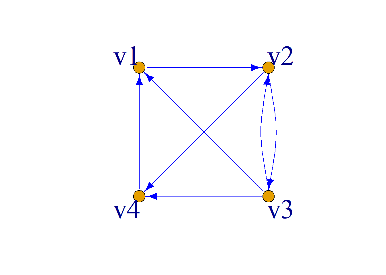
\[ B_4=\sum_{i=1}^4A^i= \left( \begin{aligned} 3&4&2&3\\ 5&{5}&4&6\\ 7&7&\boxed{4}&7\\ 3&\boxed{2}&1&2\\ \end{aligned} \right) \]
There are 2 walks from \(v_4\) to \(v_2\) of length at most 4; there are 4 cycles at \(v_3\) of length at most 4.
Definition: Let \(G={\langle}V, E{\rangle}\) be a simple directed graph, \(V=\{v_1, v_2, {\cdots}, v_n\}\), then the \(n{\times}n\) matrix \(p=(p_{ij})_{n{\times}n}\) is called the reachability matrix of \(G\), where:
\[ p_{ij}= \begin{cases} 1 & \text{if } v_i \text{ can reach } v_j \\ 0 & \text{if } v_i \text{ cannot reach } v_j \\ \end{cases} \]
Reachability matrix: \[P= \left( \begin{aligned} 1&0&0&0&1\\ 1&1&0&0&1\\ 1&1&1&1&1\\ 0&0&0&1&1\\ 0&0&0&0&1\\ \end{aligned} \right) \]
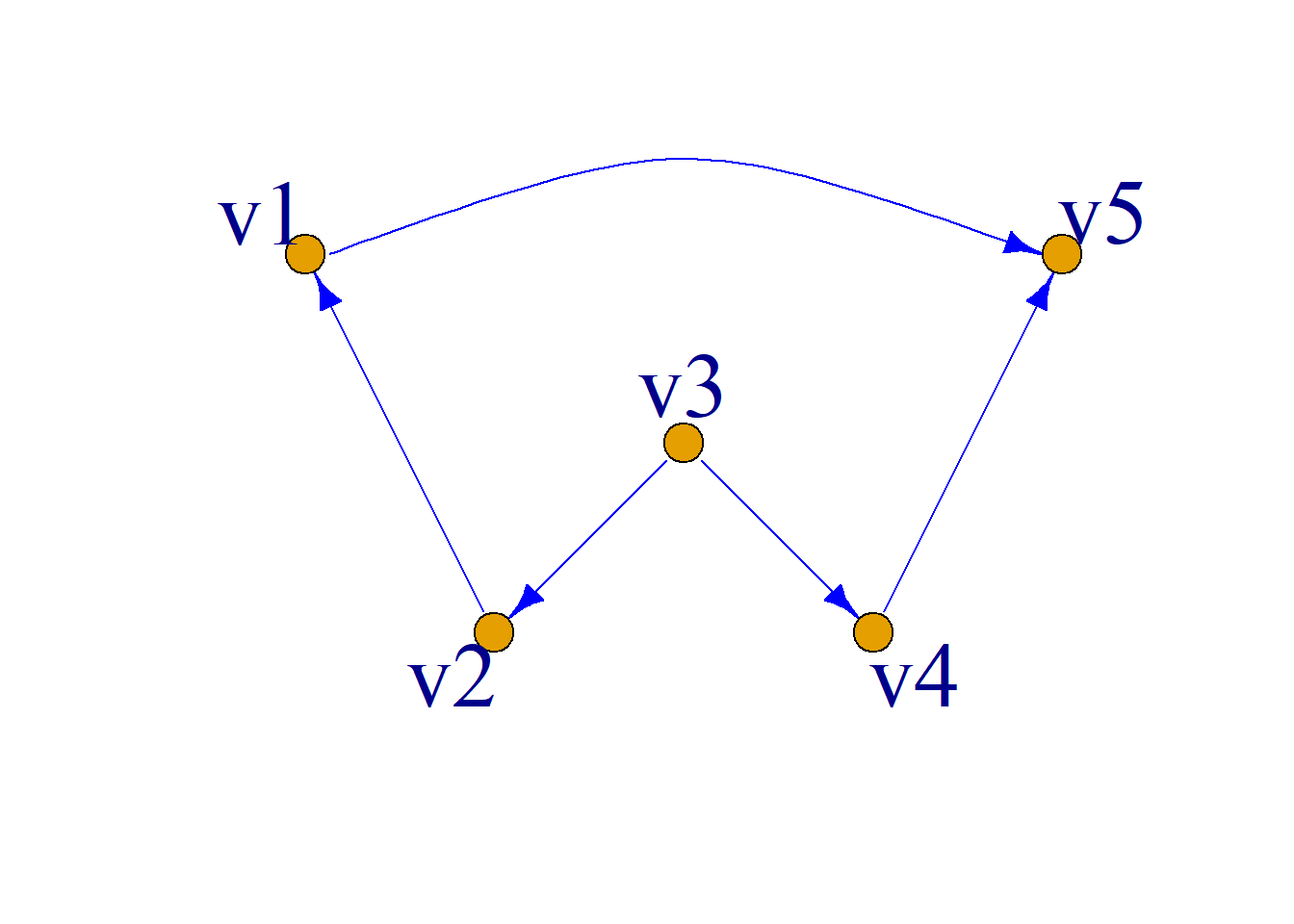
Algorithm to compute the reachability matrix \(P\) from adjacency matrix \(A\): Compute the matrix: \[B_{n-1}=(b_{ij}^{(n-1)})_{n{\times}n}=A+A^2+{\cdots}+A^{n-1}\] From matrix \(B_{n-1}\), the reachability matrix \(P=(p_{ij})_{n{\times}n}\) can be obtained. \[ p_{ij}= \begin{cases} 1 & i=j \\ 1 & i{\neq}j, b_{ij}^{(n-1)}{\neq}0 \\ 0 & i{\neq}j, b_{ij}^{(n-1)}=0 \\ \end{cases} \]
Since every vertex can always reach itself, define the diagonal elements \(p_{ii}=1\) (\(i=1, 2, {\cdots}, n\)).
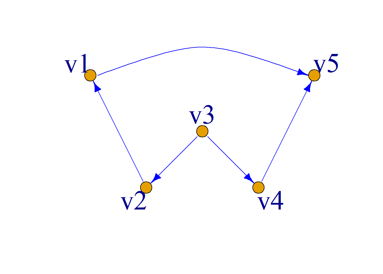
\[A= \left( \begin{aligned} 0&0&0&0&1\\ 1&0&0&0&0\\ 0&1&0&1&0\\ 0&0&0&0&1\\ 0&0&0&0&0\\ \end{aligned} \right) \] \[ A^2= \left( \begin{aligned} 0&0&0&0&0\\ 0&0&0&0&1\\ 1&0&0&0&1\\ 0&0&0&0&0\\ 0&0&0&0&0\\ \end{aligned} \right) \]
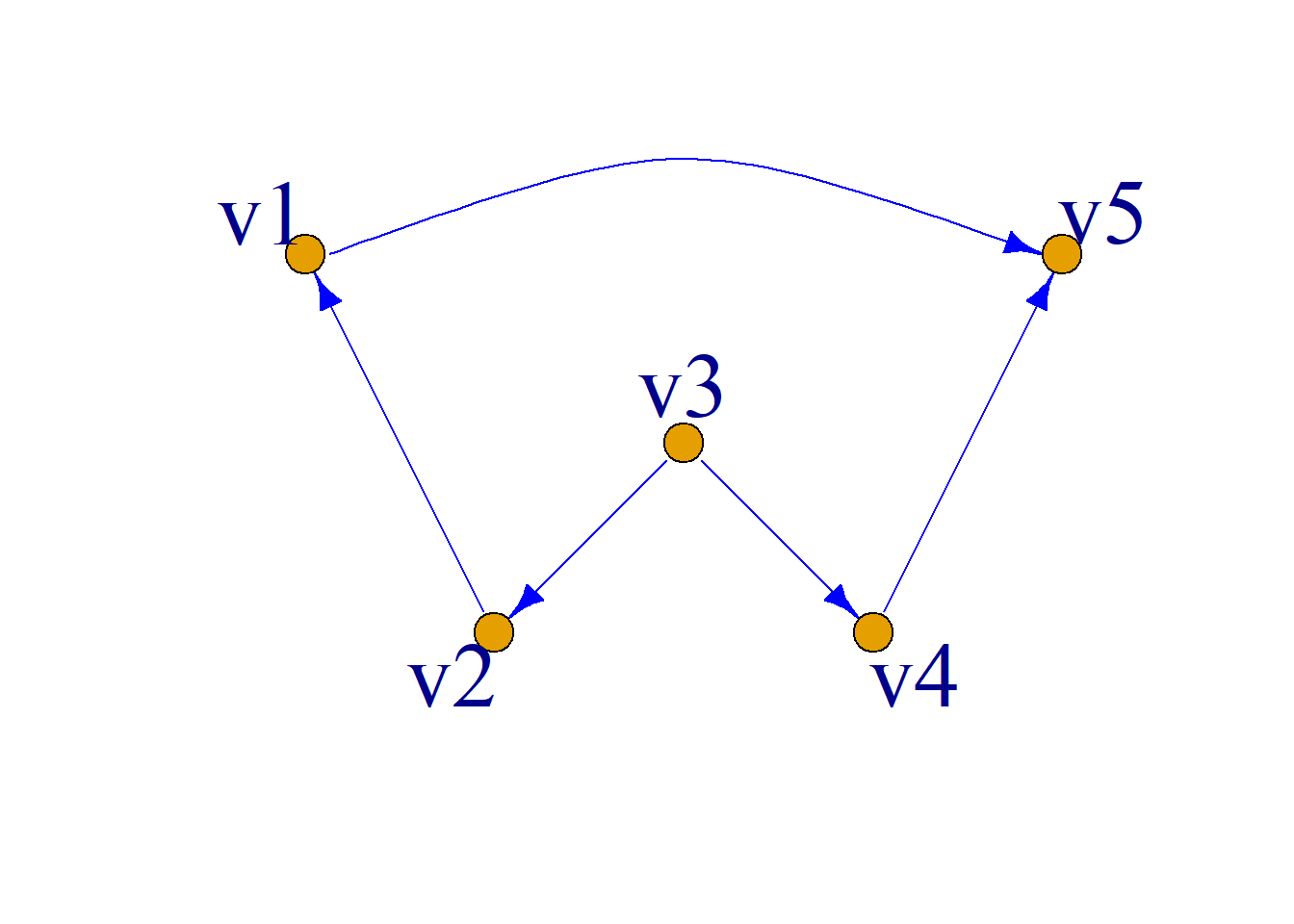
\[A^3= \left( \begin{aligned} 0&0&0&0&0\\ 0&0&0&0&0\\ 0&0&0&0&1\\ 0&0&0&0&0\\ 0&0&0&0&0\\ \end{aligned} \right) \] \[ A^4= \left( \begin{aligned} 0&0&0&0&0\\ 0&0&0&0&0\\ 0&0&0&0&0\\ 0&0&0&0&0\\ 0&0&0&0&0\\ \end{aligned} \right) \]
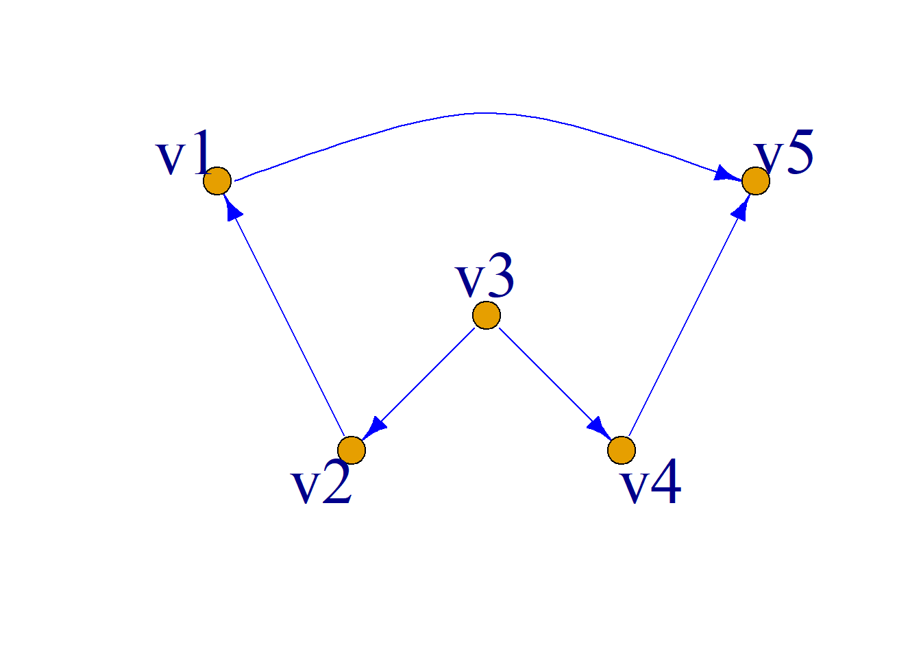
\[B_4=\sum{A^i}= \left( \begin{aligned} 0&0&0&0&1\\ 1&0&0&0&1\\ 1&1&0&1&2\\ 0&0&0&0&1\\ 0&0&0&0&0\\ \end{aligned} \right) \] Thus: \[P= \left( \begin{aligned} 1&0&0&0&1\\ 1&1&0&0&1\\ 1&1&1&1&1\\ 0&0&0&1&1\\ 0&0&0&0&1\\ \end{aligned} \right) \]
The reachability matrix and strongly connected components can be computed using Boolean matrices.
Boolean operations involve only the digits 0 and 1. Their join and meet are defined as follows: \[0{\vee}0=0, \, 0{\vee}1=1,\,1{\vee}0=1, \, 1{\vee}1=1\] \[0{\wedge}0=0, \, 0{\wedge}1=0,\,1{\wedge}0=0, \, 1{\wedge}1=1\] \({\vee}\) is called Boolean join, and \({\wedge}\) is called Boolean meet.
Boolean matrix operations: Let \(B=(b_{ij})_{n{\times}n}\) and \(C=(c_{ij})_{n{\times}n}\) be Boolean matrices. The Boolean join \(B{\vee}C\), Boolean meet \(B{\wedge}C\), and Boolean product \(B{\cdot}C\) are defined as: \[B{\vee}C=(b_{ij}{\vee}c_{ij})_{n{\times}n},\,\,B{\wedge}C=(b_{ij}{\wedge}c_{ij})_{n{\times}n},\,\,B{\cdot}C=(d_{ij})_{n{\times}n} \] where: \(d_{ij}=(b_{i1}{\wedge}c_{1j}){\vee}(b_{i2}{\wedge}c_{2j}){\vee}{\cdots}{\vee}(b_{in}{\wedge}c_{nj})\).
Given: \[ A=\left( \begin{aligned} 1&1&0\\ 0&1&0\\ 1&0&0\\ \end{aligned} \right) \, \, \, \, B=\left( \begin{aligned} 0&0&0\\ 1&1&0\\ 1&0&1\\ \end{aligned} \right) \]
Then
\[ A{\vee}B=\left( \begin{aligned} 1&1&0\\ 1&1&0\\ 1&0&0\\ \end{aligned} \right) \, \, \, \, A{\wedge}B=\left( \begin{aligned} 0&0&0\\ 0&1&0\\ 1&0&1\\ \end{aligned} \right) \, \, \, \, A{\cdot}B=\left( \begin{aligned} 1&1&0\\ 1&1&0\\ 0&0&0\\ \end{aligned} \right) \]
Let \(A\) be the adjacency matrix of a simple directed graph with \(n\) vertices. Define: \[A^{2}=A{\cdot}A\] \[A^{3}=A^{2}{\cdot}A\] \[{\cdots}\] \[A^{l}=A^{l-1}{\cdot}A\]
Then the reachability matrix of \(A\) can be expressed as: \[P=I{\vee}A{\vee}A^{2}{\vee}{\cdots}{\vee}A^{n-1}\]
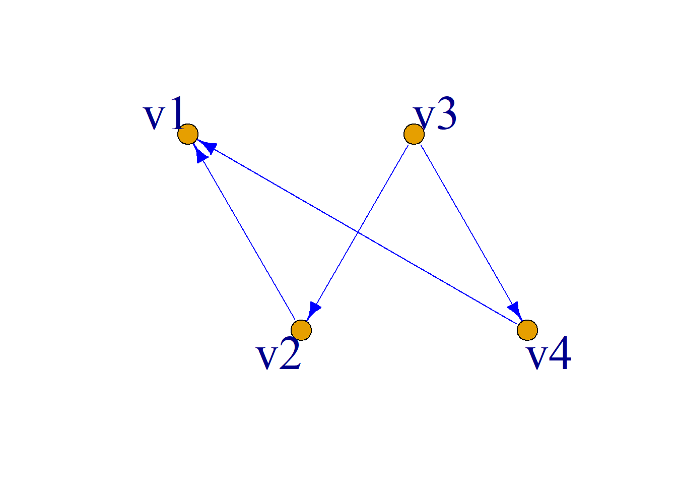
Example: Given simple directed graph \(G\) as shown, find \(P\).
Solution: \(n=4\), \(n-1=3\)
\[ A= \left( \begin{aligned} 0&0&0&0\\ 1&0&0&0\\ 0&1&0&1\\ 1&0&0&0\\ \end{aligned} \right) \] \[P=I{\vee}A{\vee}A^2{\vee}A^3\]
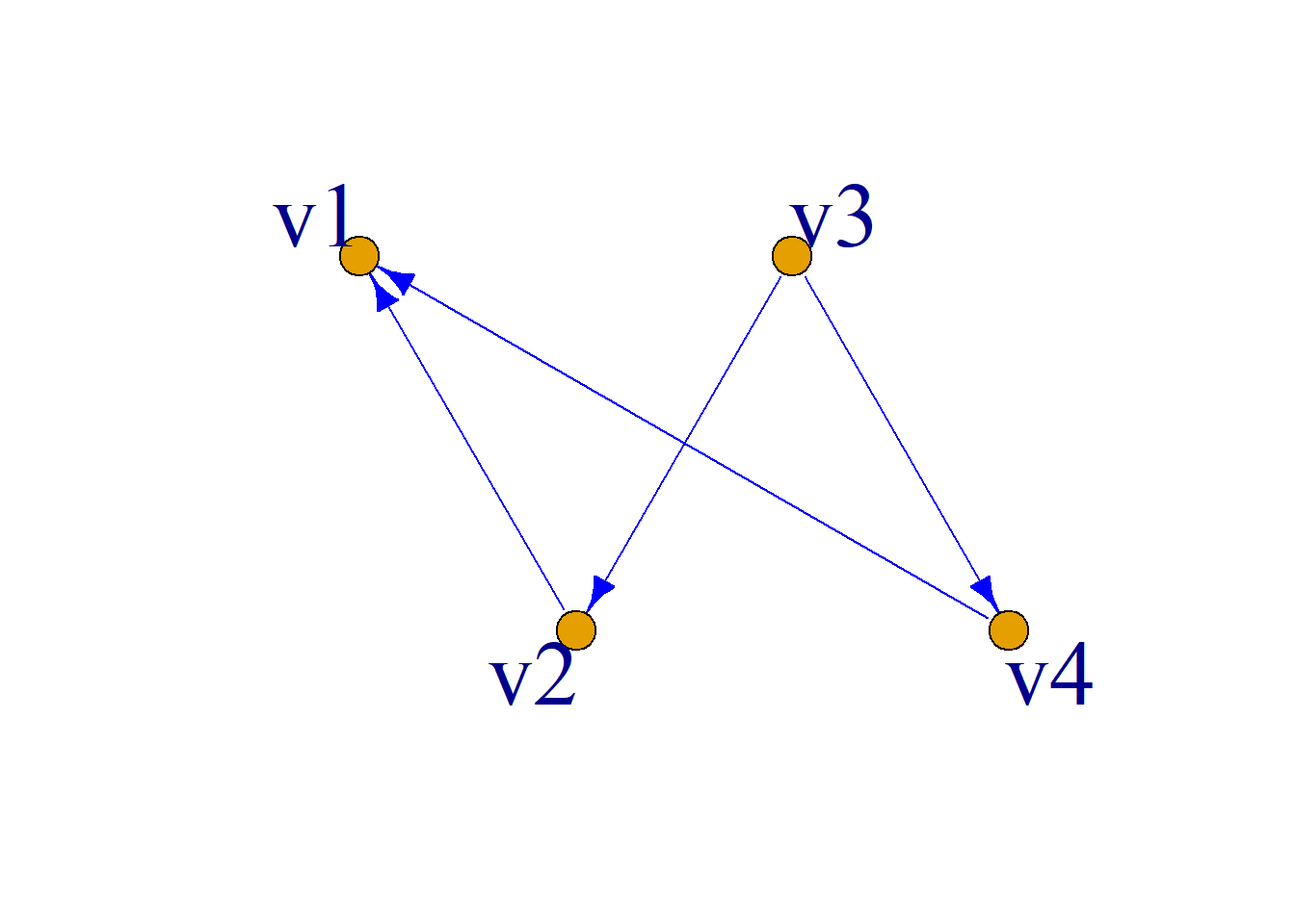
\[ A^2= \left( \begin{aligned} 0&0&0&0\\ 0&0&0&0\\ 1&0&0&0\\ 0&0&0&0\\ \end{aligned} \right) \, \, \, \, A^3={0} \]
\[ P= \left( \begin{aligned} 1&0&0&0\\ 1&1&0&0\\ 1&1&1&1\\ 1&0&0&1\\ \end{aligned} \right) \]
For simple directed graphs, the strongly connected components containing any specified vertex can be found using the reachability matrix.
Algorithm: Let \(G={\langle}V, E{\rangle}\) be a simple directed graph, \(P=(p_{ij})_{n{\times}n}\) its reachability matrix, and \(P^T=(p_{ij})^T_{n{\times}n}\) the transpose of \(P\). For the matrix
\[P{\wedge}P^T=(p_{ij}{\wedge}p_{ji})_{n{\times}n}, \]
the vertices \(v_j\) corresponding to nonzero elements in row \(i\), together with \(v_i\), form the strongly connected component containing \(v_i\).
\[ P= \left( \begin{aligned} 1&1&1&0\\ 1&1&1&0\\ 1&1&1&0\\ 1&1&1&1\\ \end{aligned} \right) \] \[ P{\wedge}P^T= \left( \begin{aligned} 1&1&1&0\\ 1&1&1&0\\ 1&1&1&0\\ 0&0&0&1\\ \end{aligned} \right) \]
Thus, \(G[\{v_1, v_2, v_3\}]\) and \(G[\{v_4\}]\) are strongly connected components.